Linear Discriminant Analysis ( LDA) with Scikit

Linear Discriminant Analysis (LDA) is similar to Principal Component Analysis (PCA) in reducing the dimensionality. However, there are certain nuances with LDA that we should be aware of-

  • LDA is supervised (needs categorical dependent variable) to provide the best linear combination of original variables while providing the maximum separation among the different groups. On the other hand, PCA is unsupervised
  • LDA can be used for classification also, whereas PCA is generally used for unsupervised learning
  • LDA doesn’t need the numbers of discriminant to be passed on ahead of time. Generally speaking the number of discriminant will be lower of the number of variables or number of categories-1.
  • LDA is more robust and can be conducted without even standardizing or normalizing the variables in certain cases
  • LDA is preferred for bigger data sets and machine learning

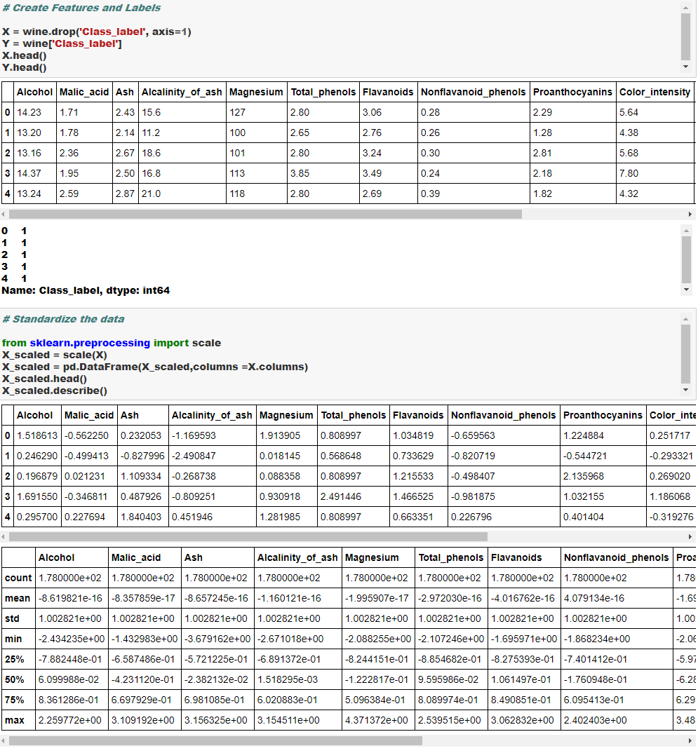
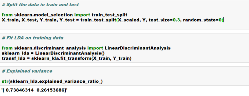
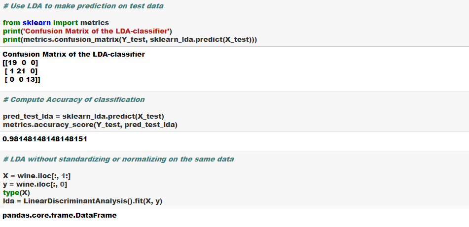
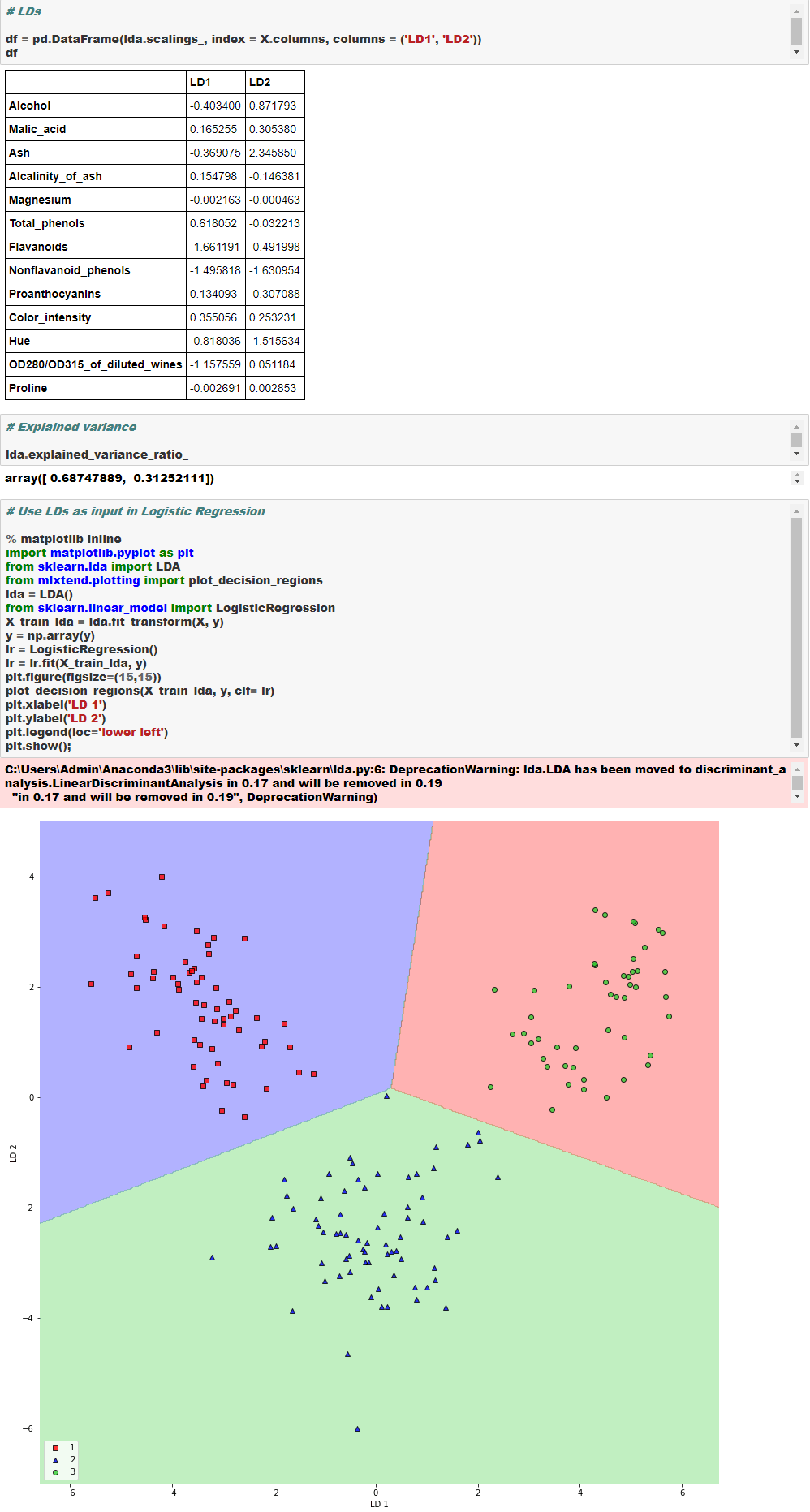
Let the action begin now-

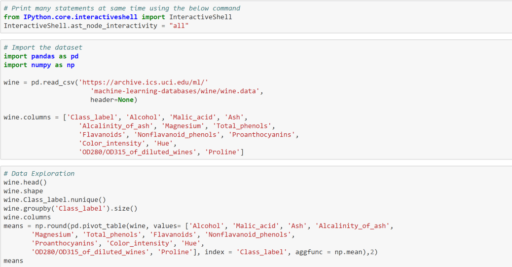
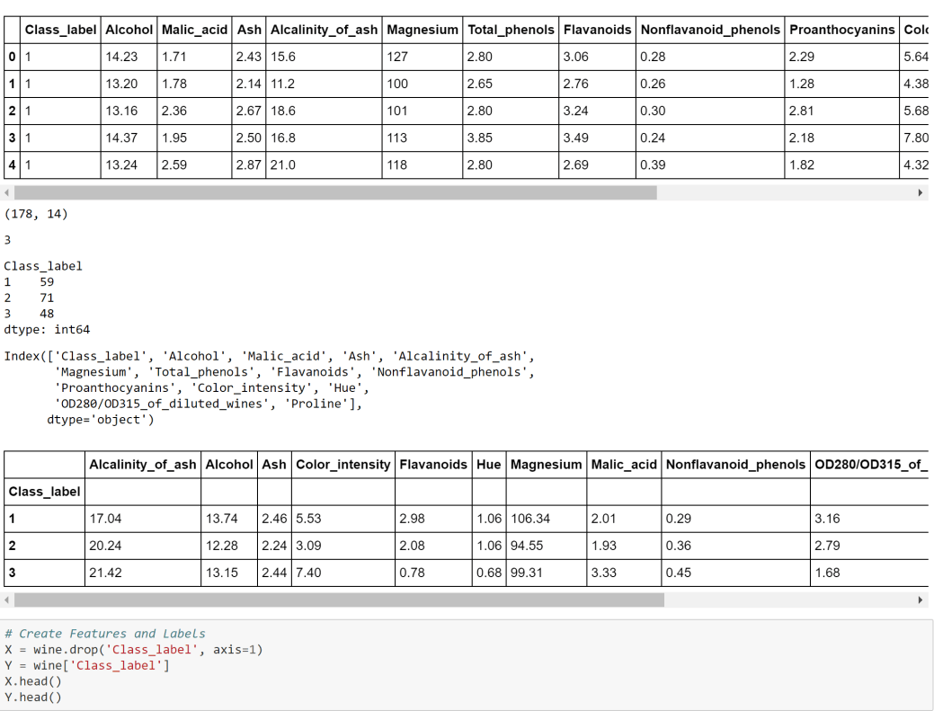
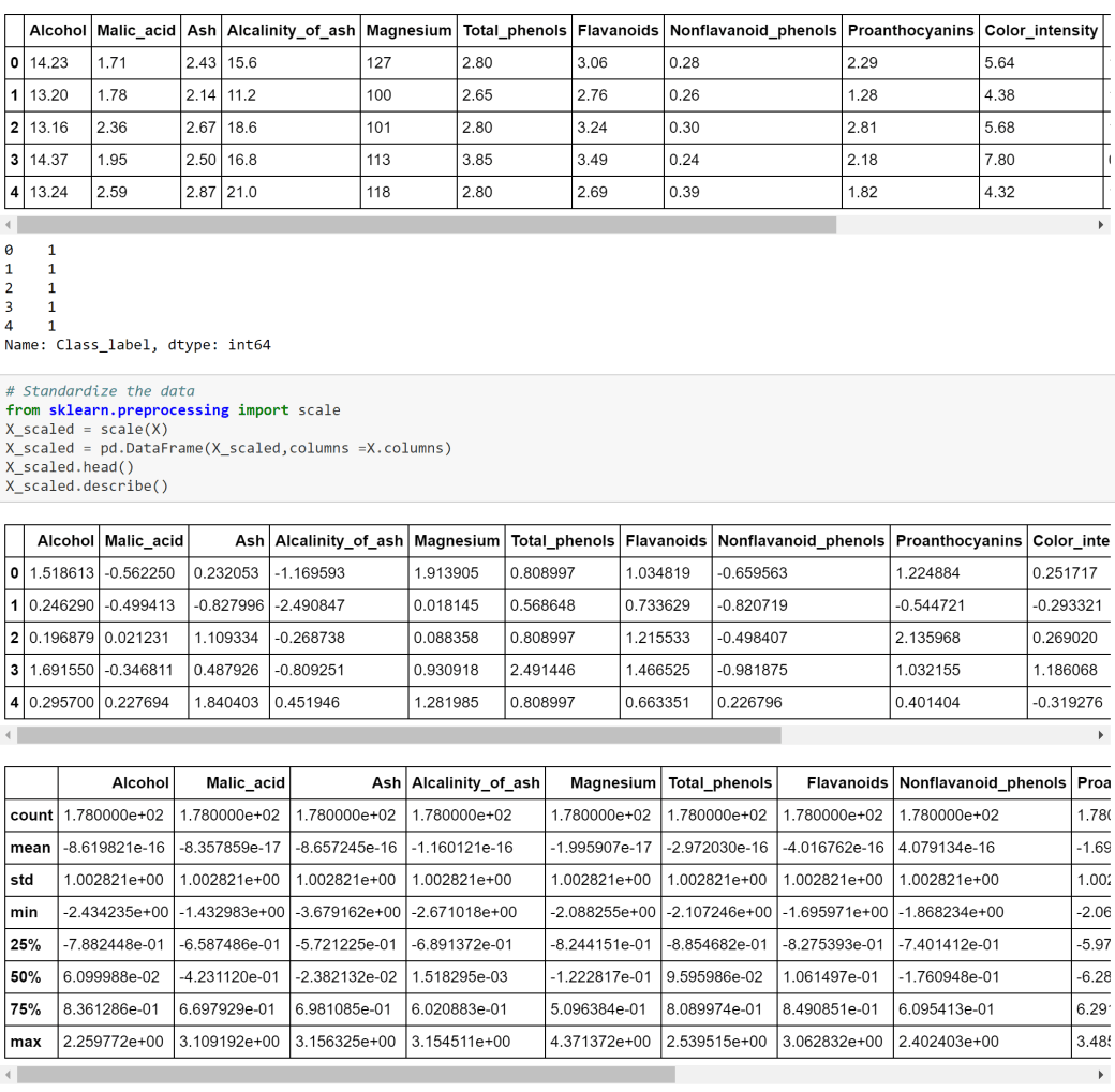
lda1LDA2LDA3LDA4LDA5

Cheers!

Principal Component Analysis ( PCA) using Scikit

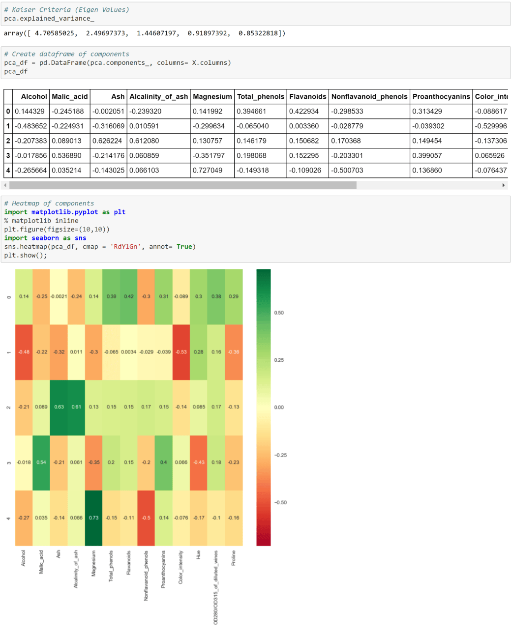
Principal Component Analysis ( PCA) is generally used as an unsupervised algorithm for reducing the data dimensions to address Curse of Dimensionality, detecting outliers, removing noise, speech recognition and other such areas.

The underlying algorithm in PCA is generally a linear algebra technique called Singular Value Decomposition (SVD). PCAs take the original data and create orthogonal components (uncorrelated components) that capture the information contained in the original data however with significantly less number of components.

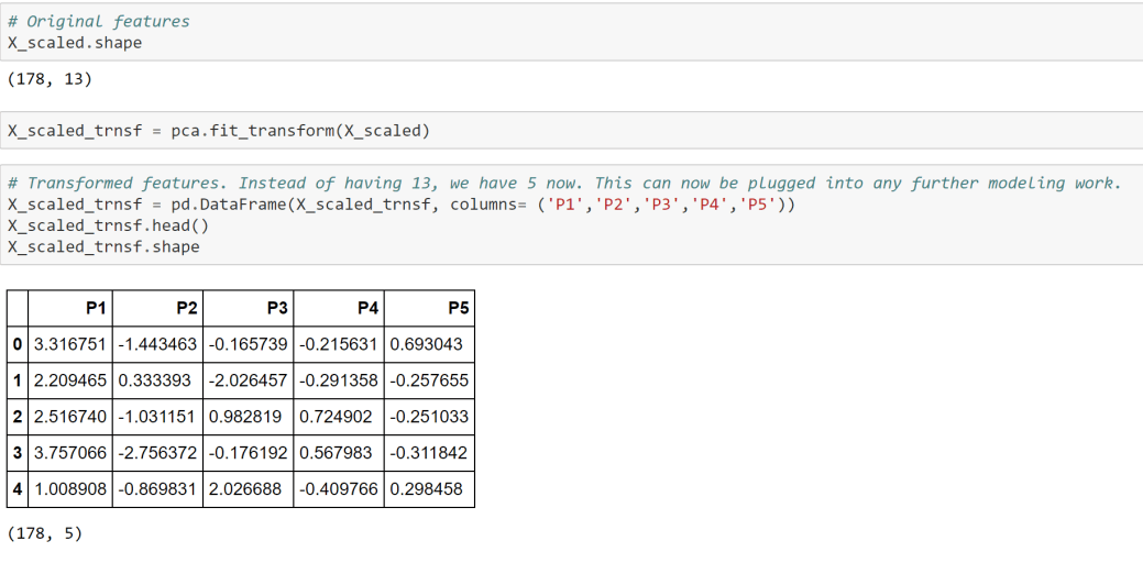
Either the components themselves or  key loading of the components can be plugged in any further modeling work, rather than the original data to minimize information redundancy and noise.

There are three main ways to select the right number of components-

  1. Number of components should explain at least 80% of the original data variance or information [Preferred One]
  2. Eigen value of each PCA component should be more than or equal to 1. This means that they should express at least one variable worth of information
  3. Elbow or Scree method- look for the elbow in the percentage of variance explained by each components and select the components where an elbow or kink is visible.

You can use any one of the above or combination of the above to select the right number of components. It is very critical to standardize or normalize data before conducting PCA.

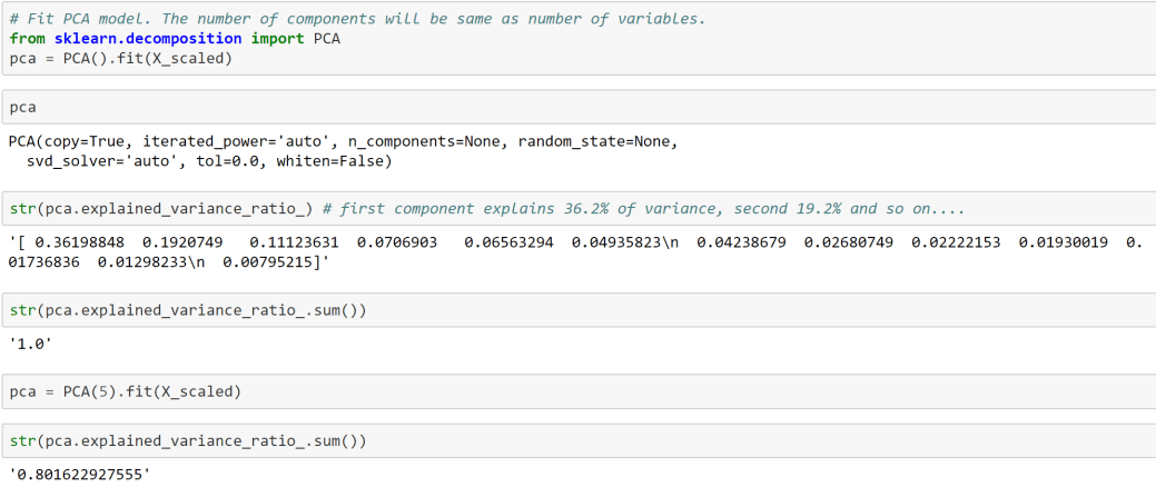
In the below case study we will use the first criterion shown above, i.e. 80% or more of the original data variance should be explained by the selected number of components.

PCA1PCA2PCA3PCA4PCA5PCA6

Logistic Regression using Scikit Python

What Is Logistic Regression?

Logistic regression is a supervised machine learning algorithm used for binary classification — predicting whether an outcome belongs to one of two classes (e.g., survived / did not survive, spam / not spam, fraud / not fraud).

Unlike linear regression, which predicts a continuous value, logistic regression predicts a probability that an observation belongs to the positive class. That probability is then converted into a class label using a decision threshold (typically 0.5).


Use Cases

Logistic regression is widely used when the target is binary or can be treated as binary:

DomainExample
HealthcareDisease diagnosis (positive / negative test result)
FinanceCredit default prediction, fraud detection
MarketingCustomer churn, click-through prediction
HREmployee attrition prediction
TransportationPassenger survival, accident severity classification

In this notebook, we use logistic regression to predict whether a Titanic passenger survived (1) or not (0) based on features such as age, gender, fare, and passenger class.


The Model Equation

Logistic regression starts with a linear combination of features (similar to linear regression):

z = β₀ + β₁x₁ + β₂x₂ + … + βₙxₙ

This value z is passed through the sigmoid (logistic) function to produce a probability between 0 and 1:

P(y = 1 | x) = σ(z) = 1 / (1 + e^(-z))

Where:

  • P(y=1 | x) = probability of the positive class
  • β₀ = intercept (bias term)
  • β₁, β₂, …, βₙ = coefficients (weights) for each feature
  • x₁, x₂, …, xₙ = input feature values

The sigmoid function squashes any real number into the range (0, 1), making it ideal for probability estimation.


Log-Odds (Logit)

Instead of modeling probability directly, logistic regression can be understood as modeling the log-odds (also called the logit) of the outcome:

logit(p) = ln(p / (1 – p)) = β₀ + β₁x₁ + β₂x₂ + … + βₙxₙ

Where:

  • p = probability of the positive class
  • p / (1-p) = odds (ratio of probability of success to probability of failure)
  • ln(p / (1-p)) = log-odds or logit

Key insight: The logit transforms a probability (bounded 0–1) into an unbounded real number, allowing us to use a linear model. A one-unit increase in a feature changes the log-odds by that feature’s coefficient βⱼ.

Example: If β_gender = 1.5, being in the coded “female” category increases the log-odds of survival by 1.5 — which corresponds to multiplying the odds by e^1.5 ≈ 4.48.


Algorithm & Optimization

Logistic regression learns the coefficients β₀, β₁, …, βₙ by maximizing the likelihood of observing the actual training labels — equivalent to minimizing the log-loss (cross-entropy loss):

L = -(1/N) × Σ [ yᵢ log(p̂ᵢ) + (1 – yᵢ) log(1 – p̂ᵢ) ]

Where:

  • N = number of training samples
  • yᵢ = actual label (0 or 1) for sample i
  • p̂ᵢ = predicted probability for sample i

How optimization works:

  1. Initialize coefficients (often to zero or small random values)
  2. Compute predicted probabilities using the sigmoid function
  3. Calculate the loss (log-loss) across all training samples
  4. Compute the gradient (partial derivatives of loss w.r.t. each coefficient)
  5. Update coefficients using an iterative solver such as:
    • L-BFGS (Limited-memory Broyden–Fletcher–Goldfarb–Shanno) — default in scikit-learn
    • Stochastic Gradient Descent (SGD)
    • Newton’s method
  6. Repeat until convergence (loss stops improving)

scikit-learn’s LogisticRegression() uses these solvers under the hood — no manual gradient descent is needed.


Underlying Assumptions

Logistic regression performs best when these assumptions are reasonably met:

AssumptionDescription
Binary outcomeThe dependent variable has only two meaningful classes
Independence of observationsEach row is independent (no repeated measures on the same subject)
Linearity of log-oddsThe log-odds of the outcome is a linear function of the predictors
No perfect multicollinearityPredictors should not be perfectly correlated with each other
Large enough sample sizeRule of thumb: at least 10 events per predictor variable
No extreme outliersOutliers can disproportionately influence coefficient estimates

Violations don’t always make the model unusable, but they can reduce accuracy or make coefficients harder to interpret.


Interpreting Coefficients

Coefficient signMeaning
Positive βⱼIncreases the log-odds (and probability) of the positive class
Negative βⱼDecreases the log-odds (and probability) of the positive class
Magnitudeβⱼ

After training, we examine log.coef_ in this notebook to see which features most strongly predict survival.


Decision Threshold & Probability Output

By default, scikit-learn classifies an observation as class 1 if P(y=1) >= 0.5, otherwise class 0. This threshold can be adjusted:

  • Lower threshold (e.g., 0.3) → more positive predictions (higher recall, lower precision)
  • Higher threshold (e.g., 0.7) → fewer positive predictions (higher precision, lower recall)

predict_proba() returns the raw probabilities, which we use later in this notebook for threshold optimization and detailed prediction analysis.


Logistic Regression vs. Linear Regression

Logistic Regression vs. Linear Regression

AspectLinear RegressionLogistic Regression
OutputContinuous valueProbability (0 to 1)
Link functionIdentitySigmoid (logit)
Loss functionMean Squared ErrorLog-loss (cross-entropy)
Use casePredicting quantitiesBinary classification

Strengths & Limitations

Strengths:

  • Simple, fast, and highly interpretable
  • Outputs well-calibrated probabilities
  • Works well as a baseline classifier
  • Less prone to overfitting with small datasets (with regularization)

Limitations:

  • Assumes a linear decision boundary in log-odds space
  • Struggles with complex non-linear relationships
  • Sensitive to feature scaling (we apply StandardScaler in this notebook)
  • Requires thoughtful handling of missing values and categorical encoding

CODES

# =============================================================================
# IMPORTS AND ENVIRONMENT SETUP
# =============================================================================
# Import core libraries for numerics, data handling, and plotting
import numpy as np
import pandas as pd
from matplotlib import pyplot as plt
import seaborn as sns
#import pandas_profiling
%matplotlib inline
!pip install tqdm

# Enable multiple expressions per cell in Jupyter (shows all results, not just last)
from IPython.core.interactiveshell import InteractiveShell
InteractiveShell.ast_node_interactivity = “all”


# =============================================================================
# EXPLORATORY DATA ANALYSIS — Titanic Dataset Overview
# =============================================================================
# Load a fresh copy of the Titanic dataset for initial exploration
titanic_eda = sns.load_dataset(‘titanic’)

# — Dataset shape and basic statistics —
print(“=” * 60)
print(“TITANIC DATASET — EXPLORATORY DATA ANALYSIS”)
print(“=” * 60)
print(f”\nDataset Shape: {titanic_eda.shape[0]} rows x {titanic_eda.shape[1]} columns”)
print(f”Overall Survival Rate: {titanic_eda[‘survived’].mean():.1%}”)
print(“\n— Missing Values —“)
print(titanic_eda.isna().sum())
print(“\n— Survival by Gender —“)
print(titanic_eda.groupby(‘sex’)[‘survived’].mean().round(3))
print(“\n— Survival by Passenger Class —“)
print(titanic_eda.groupby(‘pclass’)[‘survived’].mean().round(3))

# — Chart 1: Overview panel (survival, gender, class, age) —
fig, axes = plt.subplots(2, 2, figsize=(14, 10))

sns.countplot(data=titanic_eda, x=’survived’, ax=axes[0, 0], palette=’Set2′)
axes[0, 0].set_title(‘Survival Count (0 = Died, 1 = Survived)’)
axes[0, 0].set_xlabel(‘Survived’)

sns.countplot(data=titanic_eda, x=’sex’, hue=’survived’, ax=axes[0, 1], palette=’Set1′)
axes[0, 1].set_title(‘Survival by Gender’)
axes[0, 1].legend(title=’Survived’)

sns.countplot(data=titanic_eda, x=’pclass’, hue=’survived’, ax=axes[1, 0], palette=’Set1′)
axes[1, 0].set_title(‘Survival by Passenger Class’)
axes[1, 0].set_xlabel(‘Passenger Class’)
axes[1, 0].legend(title=’Survived’)

sns.histplot(data=titanic_eda, x=’age’, hue=’survived’, kde=True, ax=axes[1, 1], palette=’Set1′)
axes[1, 1].set_title(‘Age Distribution by Survival Status’)

plt.suptitle(‘Titanic EDA — Key Survival Patterns’, fontsize=14, y=1.02)
plt.tight_layout()
plt.show()

# — Chart 2: Fare distribution and missing values —
fig, axes = plt.subplots(1, 2, figsize=(14, 5))

sns.boxplot(data=titanic_eda, x=’survived’, y=’fare’, ax=axes[0], palette=’Pastel1′)
axes[0].set_title(‘Fare Distribution by Survival Status’)
axes[0].set_xlabel(‘Survived (0 = Died, 1 = Survived)’)

missing = titanic_eda.isna().sum()
missing = missing[missing > 0].sort_values(ascending=False)
missing.plot(kind=’bar’, ax=axes[1], color=’coral’, edgecolor=’black’)
axes[1].set_title(‘Missing Values by Column’)
axes[1].set_ylabel(‘Count’)
axes[1].tick_params(axis=’x’, rotation=45)

plt.tight_layout()
plt.show()

# — Chart 3: Correlation heatmap for numeric features —
numeric_cols = titanic_eda.select_dtypes(include=’number’).columns
corr = titanic_eda[numeric_cols].corr()
plt.figure(figsize=(8, 6))
sns.heatmap(corr, annot=True, fmt=’.2f’, cmap=’coolwarm’, center=0, square=True)
plt.title(‘Correlation Heatmap — Numeric Features’)
plt.tight_layout()
plt.show()


# =============================================================================
# LOAD TITANIC DATA
# =============================================================================
# Load the built-in Titanic dataset from seaborn and preview first/last rows
titanic = sns.load_dataset(‘titanic’)
titanic.head()
titanic.tail()

# =============================================================================
# PROGRESS BAR DEMO (tqdm)
# =============================================================================
# Demonstrate tqdm progress bar utility
from tqdm import tqdm
from time import sleep
with tqdm(total=100) as pbar:
for i in range(10):
sleep(0.1)
pbar.update(10)

# =============================================================================
# DROP REDUNDANT / LEAKAGE COLUMNS
# =============================================================================
# Remove columns that duplicate information or would leak the target variable
# Note: ‘deck’ is kept here because it is imputed later in the missing-value section
titanic.drop([‘alive’, ‘class’,’who’, ’embark_town’, ‘alone’, ‘adult_male’]
,axis=1,inplace=True)


# Preview cleaned dataframe
titanic.head()

# Check data types and non-null counts
titanic.info()

# Explore embarked port distribution before handling missing values
titanic[’embarked’].value_counts()

# Find the most frequent embarkation port (used for imputation)
titanic[’embarked’].mode()

# Inspect rows with missing embarked values
titanic.iloc[[61,684],:]

titanic.info()

# Fill missing embarked values with the mode (most common port: Southampton)
titanic[’embarked’] = titanic[’embarked’].fillna(titanic[’embarked’].mode()[0])

titanic.info()

# Summary of remaining missing values across all columns
titanic.isna().sum()

titanic.shape

# =============================================================================
# REMOVE DUPLICATE ROWS
# =============================================================================
# drop duplicates
titanic = titanic.drop_duplicates()
titanic.shape

# =============================================================================
# EXPLORE MISSING AGE VALUES
# =============================================================================
# Isolate passengers with missing age for inspection
titanic_age_missing = titanic[titanic[‘age’].isna()]
titanic_age_missing.head()
titanic_age_missing.shape

# Inspect specific rows of interest
titanic.iloc[[19,26,28],:]

# =============================================================================
# RENAME COLUMNS FOR CLARITY
# =============================================================================
# Standardize column names to descriptive lowercase labels
titanic = titanic.rename(columns = {“sex”:”gender”, “sibsp”:’siblings_spouse’,
“parch”:”parents_child”,”Survived”:’survived’,
“Pclass”:’plcass’,
‘Age’:’age’,’Fare’:’fare’, ‘Embarked’:’embarked’})
titanic.head()

titanic.info()

titanic.columns

titanic[’embarked’].value_counts()

# =============================================================================
# DECK COLUMN — MISSING VALUE TREATMENT
# =============================================================================
# Convert deck to object type and fill missing deck values with ‘Not Assigned’
# (Must run before categorical encoding so deck is not dropped and median fill works)
titanic.deck = titanic.deck.astype(‘object’)

titanic[‘deck’] = titanic[‘deck’].fillna(‘Not Assigned’)

titanic.info()

titanic.deck.isna().sum()

# =============================================================================
# ENCODE CATEGORICAL VARIABLES AS INTEGER CODES
# =============================================================================
# Convert object-type columns to numeric category codes for modeling
for x in titanic.columns:
if titanic[x].dtype == “object”:
titanic[x]=pd.Categorical(titanic[x]).codes

titanic.head()

# =============================================================================
# IMPUTE MISSING AGE WITH MEDIAN
# =============================================================================
# Compute median age and fill missing age values
titanic[‘age’].median()

titanic[‘age’] = titanic[‘age’].fillna(titanic[‘age’].median())
titanic.info()

# Fill any remaining numeric missing values with column medians
titanic= titanic.fillna(titanic.median())
titanic.info()

titanic.iloc[[19,26,28],:]

# =============================================================================
# HANDLE REMAINING EMBARKED MISSING VALUES
# =============================================================================
titanic_embark_missing = titanic[titanic[’embarked’].isna()]
titanic_embark_missing

titanic[’embarked’].mode()

titanic[’embarked’] = titanic[’embarked’].fillna(titanic[’embarked’].mode()[0])

titanic.iloc[[61,684],:]

# Sample and inspect the cleaned dataset
titanic.head(10)
titanic.sample(10)
titanic.tail(10)
titanic.info()

titanic.columns

titanic.info()

# =============================================================================
# DESCRIPTIVE STATISTICS AND OUTLIER ANALYSIS
# =============================================================================
# Summary statistics for all numeric columns
titanic.describe()

# Percentile distribution to identify potential outliers
titanic.quantile((0, 0.01,0.05, 0.5, 0.95,0.99, 1.0))

# Visualize fare distribution before clipping outliers
titanic.fare.hist()


# Clip fare outliers at the 99th percentile upper bound
titanic.fare = np.clip(titanic.fare,0,249.00622 )

titanic.fare.describe()

titanic.fare.hist()

titanic.info()

titanic.describe()

# Clip all numeric columns to their 1st and 99th percentile bounds
for x in titanic.columns:
outlier = titanic[x].quantile([0.01,0.99]).values
titanic[x] = np.clip(titanic[x], outlier[0], outlier[1])


titanic.describe()

# prompt: read a csv file

#df = pd.read_csv(‘filename.csv’)


titanic.describe()
titanic.head()

# Check class balance of the target variable (survived)
titanic.groupby(‘survived’).size()

titanic.shape

# =============================================================================
# PREPARE FEATURES (X) AND TARGET (y)
# =============================================================================
# Import scikit-learn modules for splitting, metrics, and logistic regression
from sklearn.model_selection import train_test_split
from sklearn import metrics
from sklearn.linear_model import LogisticRegression


# Separate features from target variable
x = titanic.drop([‘survived’], axis = 1, inplace=False)
y = titanic[‘survived’]
x.shape
print(‘\n’)
y.shape

titanic.describe()

# =============================================================================
# FEATURE SCALING — MinMaxScaler (demonstration)
# =============================================================================
from sklearn.preprocessing import MinMaxScaler
scld_titanic = MinMaxScaler(feature_range= (0,1))
titanic_transformed = scld_titanic.fit_transform(x)
scld_titanic_df = pd.DataFrame(titanic_transformed, columns = x.columns)
scld_titanic_df.head()
scld_titanic_df.describe()

# =============================================================================
# FEATURE SCALING — StandardScaler (used for modeling)
# =============================================================================
from sklearn.preprocessing import StandardScaler
scld_titanic = StandardScaler()
titanic_transformed = scld_titanic.fit_transform(x)
scld_titanic_df = pd.DataFrame(titanic_transformed, columns = x.columns)
scld_titanic_df.head()
np.round(scld_titanic_df.describe(),2)

# =============================================================================
# TRAIN / TEST SPLIT
# =============================================================================
# Split in Train and Test data
x_train, x_test, y_train, y_test = train_test_split(scld_titanic_df, y, test_size=0.2, random_state=999)
x_train.shape
y_train.shape
x_test.shape
y_test.shape

x_train
y_train
x_test

# Check survival rate (% positive class) in train and test sets
np.round(y_train.sum()/y_train.count()*100,2)
print(‘\n’)
np.round(y_test.sum()/y_test.count()*100,2)

# =============================================================================
# LOGISTIC REGRESSION MODEL
# =============================================================================
# Initialize logistic regression classifier
log = LogisticRegression()

log

# Fit the model on training data
log.fit(x_train, y_train)

# =============================================================================
# PREDICTIONS AND EVALUATION
# =============================================================================
# Generate class predictions on the test set
predicted = log.predict(x_test)
predicted

from sklearn import metrics
print((metrics.classification_report(y_test, predicted)))

# Build confusion matrix comparing actual vs predicted labels
df_confusion = metrics.confusion_matrix(y_test,predicted)
df_confusion


import seaborn as sns
import matplotlib.pyplot as plt
# Visualize confusion matrix as a heatmap
sns.heatmap(df_confusion, cmap = ‘Greens’,xticklabels=[‘Prediction No’,’Prediction Yes’],
yticklabels=[‘Actual No’,’Actual Yes’], annot=True, fmt=’d’)
plt.show();

# Overall accuracy score
metrics.accuracy_score(y_test, predicted)

# =============================================================================
# MODEL INTERPRETATION — COEFFICIENTS
# =============================================================================
# Raw model coefficients (log-odds impact of each feature)
log.coef_

x.columns

# Combine feature names with their coefficients for readability
coeff = pd.concat([pd.DataFrame(x.columns), pd.DataFrame(np.transpose(log.coef_))],axis =1 )
coeff.columns = (“Variable”, ‘Coeff’)

coeff

# =============================================================================
# PROBABILITY PREDICTIONS AND THRESHOLD ANALYSIS
# =============================================================================
# Find out probability of the classes and predicted classes
predicted_prob = log.predict_proba(x_test)
predicted_prob_df = pd.DataFrame(predicted_prob)
predicted_classes_df = pd.DataFrame(predicted)
y_actual_df = pd.DataFrame(y_test.values)
predicted_df = pd.concat([predicted_prob_df, predicted_classes_df, y_actual_df], axis=1)
predicted_df.columns = [‘Prob_0′,’Prob_1′,’Predicted_Class’, ‘Actual_Class’]
predicted_df.sample(20)


predicted_prob

Output Block

Requirement already satisfied: tqdm in /usr/local/lib/python3.12/dist-packages (4.67.3)
============================================================
TITANIC DATASET — EXPLORATORY DATA ANALYSIS
============================================================

Dataset Shape: 891 rows x 15 columns
Overall Survival Rate: 38.4%

— Missing Values —
survived 0
pclass 0
sex 0
age 177
sibsp 0
parch 0
fare 0
embarked 2
class 0
who 0
adult_male 0
deck 688
embark_town 2
alive 0
alone 0
dtype: int64

— Survival by Gender —
sex
female 0.742
male 0.189
Name: survived, dtype: float64

— Survival by Passenger Class —
pclass
1 0.630
2 0.473
3 0.242
Name: survived, dtype: float64
/tmp/ipykernel_597/1527970602.py:40: FutureWarning:

Passing `palette` without assigning `hue` is deprecated and will be removed in v0.14.0. Assign the `x` variable to `hue` and set `legend=False` for the same effect.

sns.countplot(data=titanic_eda, x=’survived’, ax=axes[0, 0], palette=’Set2′)

/tmp/ipykernel_597/1527970602.py:63: FutureWarning:

Passing `palette` without assigning `hue` is deprecated and will be removed in v0.14.0. Assign the `x` variable to `hue` and set `legend=False` for the same effect.

sns.boxplot(data=titanic_eda, x=’survived’, y=’fare’, ax=axes[0], palette=’Pastel1′)


100%|██████████| 100/100 [00:01<00:00, 98.40it/s]
<class ‘pandas.core.frame.DataFrame’>
RangeIndex: 891 entries, 0 to 890
Data columns (total 9 columns):
# Column Non-Null Count Dtype
— —— ————– —–
0 survived 891 non-null int64
1 pclass 891 non-null int64
2 sex 891 non-null object
3 age 714 non-null float64
4 sibsp 891 non-null int64
5 parch 891 non-null int64
6 fare 891 non-null float64
7 embarked 889 non-null object
8 deck 203 non-null category
dtypes: category(1), float64(2), int64(4), object(2)
memory usage: 57.0+ KB
<class ‘pandas.core.frame.DataFrame’>
RangeIndex: 891 entries, 0 to 890
Data columns (total 9 columns):
# Column Non-Null Count Dtype
— —— ————– —–
0 survived 891 non-null int64
1 pclass 891 non-null int64
2 sex 891 non-null object
3 age 714 non-null float64
4 sibsp 891 non-null int64
5 parch 891 non-null int64
6 fare 891 non-null float64
7 embarked 889 non-null object
8 deck 203 non-null category
dtypes: category(1), float64(2), int64(4), object(2)
memory usage: 57.0+ KB
<class ‘pandas.core.frame.DataFrame’>
RangeIndex: 891 entries, 0 to 890
Data columns (total 9 columns):
# Column Non-Null Count Dtype
— —— ————– —–
0 survived 891 non-null int64
1 pclass 891 non-null int64
2 sex 891 non-null object
3 age 714 non-null float64
4 sibsp 891 non-null int64
5 parch 891 non-null int64
6 fare 891 non-null float64
7 embarked 891 non-null object
8 deck 203 non-null category
dtypes: category(1), float64(2), int64(4), object(2)
memory usage: 57.0+ KB
<class ‘pandas.core.frame.DataFrame’>
Index: 784 entries, 0 to 890
Data columns (total 9 columns):
# Column Non-Null Count Dtype
— —— ————– —–
0 survived 784 non-null int64
1 pclass 784 non-null int64
2 gender 784 non-null object
3 age 678 non-null float64
4 siblings_spouse 784 non-null int64
5 parents_child 784 non-null int64
6 fare 784 non-null float64
7 embarked 784 non-null object
8 deck 202 non-null category
dtypes: category(1), float64(2), int64(4), object(2)
memory usage: 56.2+ KB
<class ‘pandas.core.frame.DataFrame’>
Index: 784 entries, 0 to 890
Data columns (total 9 columns):
# Column Non-Null Count Dtype
— —— ————– —–
0 survived 784 non-null int64
1 pclass 784 non-null int64
2 gender 784 non-null object
3 age 678 non-null float64
4 siblings_spouse 784 non-null int64
5 parents_child 784 non-null int64
6 fare 784 non-null float64
7 embarked 784 non-null object
8 deck 784 non-null object
dtypes: float64(2), int64(4), object(3)
memory usage: 61.2+ KB
<class ‘pandas.core.frame.DataFrame’>
Index: 784 entries, 0 to 890
Data columns (total 9 columns):
# Column Non-Null Count Dtype
— —— ————– —–
0 survived 784 non-null int64
1 pclass 784 non-null int64
2 gender 784 non-null int8
3 age 784 non-null float64
4 siblings_spouse 784 non-null int64
5 parents_child 784 non-null int64
6 fare 784 non-null float64
7 embarked 784 non-null int8
8 deck 784 non-null int8
dtypes: float64(2), int64(4), int8(3)
memory usage: 45.2 KB
<class ‘pandas.core.frame.DataFrame’>
Index: 784 entries, 0 to 890
Data columns (total 9 columns):
# Column Non-Null Count Dtype
— —— ————– —–
0 survived 784 non-null int64
1 pclass 784 non-null int64
2 gender 784 non-null int8
3 age 784 non-null float64
4 siblings_spouse 784 non-null int64
5 parents_child 784 non-null int64
6 fare 784 non-null float64
7 embarked 784 non-null int8
8 deck 784 non-null int8
dtypes: float64(2), int64(4), int8(3)
memory usage: 45.2 KB
<class ‘pandas.core.frame.DataFrame’>
Index: 784 entries, 0 to 890
Data columns (total 9 columns):
# Column Non-Null Count Dtype
— —— ————– —–
0 survived 784 non-null int64
1 pclass 784 non-null int64
2 gender 784 non-null int8
3 age 784 non-null float64
4 siblings_spouse 784 non-null int64
5 parents_child 784 non-null int64
6 fare 784 non-null float64
7 embarked 784 non-null int8
8 deck 784 non-null int8
dtypes: float64(2), int64(4), int8(3)
memory usage: 45.2 KB
<class ‘pandas.core.frame.DataFrame’>
Index: 784 entries, 0 to 890
Data columns (total 9 columns):
# Column Non-Null Count Dtype
— —— ————– —–
0 survived 784 non-null int64
1 pclass 784 non-null int64
2 gender 784 non-null int8
3 age 784 non-null float64
4 siblings_spouse 784 non-null int64
5 parents_child 784 non-null int64
6 fare 784 non-null float64
7 embarked 784 non-null int8
8 deck 784 non-null int8
dtypes: float64(2), int64(4), int8(3)
memory usage: 45.2 KB
<class ‘pandas.core.frame.DataFrame’>
Index: 784 entries, 0 to 890
Data columns (total 9 columns):
# Column Non-Null Count Dtype
— —— ————– —–
0 survived 784 non-null int64
1 pclass 784 non-null int64
2 gender 784 non-null int8
3 age 784 non-null float64
4 siblings_spouse 784 non-null int64
5 parents_child 784 non-null int64
6 fare 784 non-null float64
7 embarked 784 non-null int8
8 deck 784 non-null int8
dtypes: float64(2), int64(4), int8(3)
memory usage: 45.2 KB


precision recall f1-score support

0 0.79 0.83 0.81 90
1 0.76 0.70 0.73 67

accuracy 0.78 157
macro avg 0.77 0.77 0.77 157
weighted avg 0.78 0.78 0.78 157


array([[0.55397344, 0.44602656],
[0.36648402, 0.63351598],
[0.82161992, 0.17838008],
[0.14546149, 0.85453851],
[0.84317581, 0.15682419],
[0.85898305, 0.14101695],
[0.1203916 , 0.8796084 ],
[0.53805585, 0.46194415],
[0.35717302, 0.64282698],
[0.32849211, 0.67150789],
[0.8049969 , 0.1950031 ],
[0.91066252, 0.08933748],
[0.14053402, 0.85946598],
[0.80303192, 0.19696808],
[0.20489829, 0.79510171],
[0.53863242, 0.46136758],
[0.83888713, 0.16111287],
[0.74881101, 0.25118899],
[0.87802515, 0.12197485],
[0.06159685, 0.93840315],
[0.27139185, 0.72860815],
[0.86190473, 0.13809527],
[0.75697559, 0.24302441],
[0.54108302, 0.45891698],
[0.44893086, 0.55106914],
[0.24285506, 0.75714494],
[0.92521486, 0.07478514],
[0.44515852, 0.55484148],
[0.91673444, 0.08326556],
[0.88859559, 0.11140441],
[0.94591075, 0.05408925],
[0.93521218, 0.06478782],
[0.62625257, 0.37374743],
[0.92211925, 0.07788075],
[0.45685666, 0.54314334],
[0.84312216, 0.15687784],
[0.88547452, 0.11452548],
[0.30936126, 0.69063874],
[0.07939955, 0.92060045],
[0.93219874, 0.06780126],
[0.63330031, 0.36669969],
[0.92053872, 0.07946128],
[0.92868217, 0.07131783],
[0.5183927 , 0.4816073 ],
[0.1146845 , 0.8853155 ],
[0.72566823, 0.27433177],
[0.48886081, 0.51113919],
[0.16107575, 0.83892425],
[0.53904267, 0.46095733],
[0.72140052, 0.27859948],
[0.62960379, 0.37039621],
[0.89962517, 0.10037483],
[0.38187136, 0.61812864],
[0.84040645, 0.15959355],
[0.83113253, 0.16886747],
[0.37034959, 0.62965041],
[0.70190266, 0.29809734],
[0.77624547, 0.22375453],
[0.43187485, 0.56812515],
[0.07140916, 0.92859084],
[0.20527775, 0.79472225],
[0.61233815, 0.38766185],
[0.88753928, 0.11246072],
[0.37644464, 0.62355536],
[0.94206494, 0.05793506],
[0.24231454, 0.75768546],
[0.38422862, 0.61577138],
[0.89253394, 0.10746606],
[0.91772881, 0.08227119],
[0.81285549, 0.18714451],
[0.42634743, 0.57365257],
[0.52135864, 0.47864136],
[0.84618193, 0.15381807],
[0.67191945, 0.32808055],
[0.24777467, 0.75222533],
[0.34002452, 0.65997548],
[0.84284584, 0.15715416],
[0.80420694, 0.19579306],
[0.32039026, 0.67960974],
[0.33664048, 0.66335952],
[0.89465304, 0.10534696],
[0.85935537, 0.14064463],
[0.58474389, 0.41525611],
[0.38899587, 0.61100413],
[0.26705897, 0.73294103],
[0.13009479, 0.86990521],
[0.20701663, 0.79298337],
[0.18618385, 0.81381615],
[0.74663678, 0.25336322],
[0.74368753, 0.25631247],
[0.58907781, 0.41092219],
[0.12987609, 0.87012391],
[0.8431743 , 0.1568257 ],
[0.18348496, 0.81651504],
[0.03473669, 0.96526331],
[0.59965075, 0.40034925],
[0.90786111, 0.09213889],
[0.40560793, 0.59439207],
[0.9645318 , 0.0354682 ],
[0.95093358, 0.04906642],
[0.23132857, 0.76867143],
[0.92231606, 0.07768394],
[0.74551094, 0.25448906],
[0.879819 , 0.120181 ],
[0.65771473, 0.34228527],
[0.10796858, 0.89203142],
[0.89633336, 0.10366664],
[0.19389314, 0.80610686],
[0.94162223, 0.05837777],
[0.58125657, 0.41874343],
[0.17418465, 0.82581535],
[0.89577491, 0.10422509],
[0.84518367, 0.15481633],
[0.80321262, 0.19678738],
[0.76732066, 0.23267934],
[0.83516388, 0.16483612],
[0.75066159, 0.24933841],
[0.2825069 , 0.7174931 ],
[0.42468534, 0.57531466],
[0.85903103, 0.14096897],
[0.5367603 , 0.4632397 ],
[0.89319696, 0.10680304],
[0.41541597, 0.58458403],
[0.91095574, 0.08904426],
[0.85926671, 0.14073329],
[0.15205884, 0.84794116],
[0.837398 , 0.162602 ],
[0.82548683, 0.17451317],
[0.10576671, 0.89423329],
[0.91733691, 0.08266309],
[0.05606322, 0.94393678],
[0.85412342, 0.14587658],
[0.93426411, 0.06573589],
[0.46850755, 0.53149245],
[0.16914952, 0.83085048],
[0.12045064, 0.87954936],
[0.88320405, 0.11679595],
[0.20782634, 0.79217366],
[0.4068325 , 0.5931675 ],
[0.41507059, 0.58492941],
[0.61600861, 0.38399139],
[0.35813055, 0.64186945],
[0.53540125, 0.46459875],
[0.60871701, 0.39128299],
[0.84317102, 0.15682898],
[0.24748414, 0.75251586],
[0.78007734, 0.21992266],
[0.91667162, 0.08332838],
[0.15029365, 0.84970635],
[0.04810056, 0.95189944],
[0.89427977, 0.10572023],
[0.56399894, 0.43600106],
[0.90422189, 0.09577811],
[0.9671217 , 0.0328783 ],
[0.93949532, 0.06050468],
[0.0861572 , 0.9138428 ],
[0.46135897, 0.53864103]])

Requirement already satisfied: tqdm in /usr/local/lib/python3.12/dist-packages (4.67.3)
============================================================
TITANIC DATASET — EXPLORATORY DATA ANALYSIS
============================================================

Dataset Shape: 891 rows x 15 columns
Overall Survival Rate: 38.4%

--- Missing Values ---
survived         0
pclass           0
sex              0
age            177
sibsp            0
parch            0
fare             0
embarked         2
class            0
who              0
adult_male       0
deck           688
embark_town      2
alive            0
alone            0
dtype: int64

--- Survival by Gender ---
sex
female    0.742
male      0.189
Name: survived, dtype: float64

--- Survival by Passenger Class ---
pclass
1    0.630
2    0.473
3    0.242
Name: survived, dtype: float64
/tmp/ipykernel_597/1527970602.py:40: FutureWarning: 

Passing `palette` without assigning `hue` is deprecated and will be removed in v0.14.0. Assign the `x` variable to `hue` and set `legend=False` for the same effect.

  sns.countplot(data=titanic_eda, x='survived', ax=axes[0, 0], palette='Set2')
/tmp/ipykernel_597/1527970602.py:63: FutureWarning: 

Passing `palette` without assigning `hue` is deprecated and will be removed in v0.14.0. Assign the `x` variable to `hue` and set `legend=False` for the same effect.

  sns.boxplot(data=titanic_eda, x='survived', y='fare', ax=axes[0], palette='Pastel1')
100%|██████████| 100/100 [00:01<00:00, 98.40it/s]
<class 'pandas.core.frame.DataFrame'>
RangeIndex: 891 entries, 0 to 890
Data columns (total 9 columns):
 #   Column    Non-Null Count  Dtype   
---  ------    --------------  -----   
 0   survived  891 non-null    int64   
 1   pclass    891 non-null    int64   
 2   sex       891 non-null    object  
 3   age       714 non-null    float64 
 4   sibsp     891 non-null    int64   
 5   parch     891 non-null    int64   
 6   fare      891 non-null    float64 
 7   embarked  889 non-null    object  
 8   deck      203 non-null    category
dtypes: category(1), float64(2), int64(4), object(2)
memory usage: 57.0+ KB
<class 'pandas.core.frame.DataFrame'>
RangeIndex: 891 entries, 0 to 890
Data columns (total 9 columns):
 #   Column    Non-Null Count  Dtype   
---  ------    --------------  -----   
 0   survived  891 non-null    int64   
 1   pclass    891 non-null    int64   
 2   sex       891 non-null    object  
 3   age       714 non-null    float64 
 4   sibsp     891 non-null    int64   
 5   parch     891 non-null    int64   
 6   fare      891 non-null    float64 
 7   embarked  889 non-null    object  
 8   deck      203 non-null    category
dtypes: category(1), float64(2), int64(4), object(2)
memory usage: 57.0+ KB
<class 'pandas.core.frame.DataFrame'>
RangeIndex: 891 entries, 0 to 890
Data columns (total 9 columns):
 #   Column    Non-Null Count  Dtype   
---  ------    --------------  -----   
 0   survived  891 non-null    int64   
 1   pclass    891 non-null    int64   
 2   sex       891 non-null    object  
 3   age       714 non-null    float64 
 4   sibsp     891 non-null    int64   
 5   parch     891 non-null    int64   
 6   fare      891 non-null    float64 
 7   embarked  891 non-null    object  
 8   deck      203 non-null    category
dtypes: category(1), float64(2), int64(4), object(2)
memory usage: 57.0+ KB
<class 'pandas.core.frame.DataFrame'>
Index: 784 entries, 0 to 890
Data columns (total 9 columns):
 #   Column           Non-Null Count  Dtype   
---  ------           --------------  -----   
 0   survived         784 non-null    int64   
 1   pclass           784 non-null    int64   
 2   gender           784 non-null    object  
 3   age              678 non-null    float64 
 4   siblings_spouse  784 non-null    int64   
 5   parents_child    784 non-null    int64   
 6   fare             784 non-null    float64 
 7   embarked         784 non-null    object  
 8   deck             202 non-null    category
dtypes: category(1), float64(2), int64(4), object(2)
memory usage: 56.2+ KB
<class 'pandas.core.frame.DataFrame'>
Index: 784 entries, 0 to 890
Data columns (total 9 columns):
 #   Column           Non-Null Count  Dtype  
---  ------           --------------  -----  
 0   survived         784 non-null    int64  
 1   pclass           784 non-null    int64  
 2   gender           784 non-null    object 
 3   age              678 non-null    float64
 4   siblings_spouse  784 non-null    int64  
 5   parents_child    784 non-null    int64  
 6   fare             784 non-null    float64
 7   embarked         784 non-null    object 
 8   deck             784 non-null    object 
dtypes: float64(2), int64(4), object(3)
memory usage: 61.2+ KB
<class 'pandas.core.frame.DataFrame'>
Index: 784 entries, 0 to 890
Data columns (total 9 columns):
 #   Column           Non-Null Count  Dtype  
---  ------           --------------  -----  
 0   survived         784 non-null    int64  
 1   pclass           784 non-null    int64  
 2   gender           784 non-null    int8   
 3   age              784 non-null    float64
 4   siblings_spouse  784 non-null    int64  
 5   parents_child    784 non-null    int64  
 6   fare             784 non-null    float64
 7   embarked         784 non-null    int8   
 8   deck             784 non-null    int8   
dtypes: float64(2), int64(4), int8(3)
memory usage: 45.2 KB
<class 'pandas.core.frame.DataFrame'>
Index: 784 entries, 0 to 890
Data columns (total 9 columns):
 #   Column           Non-Null Count  Dtype  
---  ------           --------------  -----  
 0   survived         784 non-null    int64  
 1   pclass           784 non-null    int64  
 2   gender           784 non-null    int8   
 3   age              784 non-null    float64
 4   siblings_spouse  784 non-null    int64  
 5   parents_child    784 non-null    int64  
 6   fare             784 non-null    float64
 7   embarked         784 non-null    int8   
 8   deck             784 non-null    int8   
dtypes: float64(2), int64(4), int8(3)
memory usage: 45.2 KB
<class 'pandas.core.frame.DataFrame'>
Index: 784 entries, 0 to 890
Data columns (total 9 columns):
 #   Column           Non-Null Count  Dtype  
---  ------           --------------  -----  
 0   survived         784 non-null    int64  
 1   pclass           784 non-null    int64  
 2   gender           784 non-null    int8   
 3   age              784 non-null    float64
 4   siblings_spouse  784 non-null    int64  
 5   parents_child    784 non-null    int64  
 6   fare             784 non-null    float64
 7   embarked         784 non-null    int8   
 8   deck             784 non-null    int8   
dtypes: float64(2), int64(4), int8(3)
memory usage: 45.2 KB
<class 'pandas.core.frame.DataFrame'>
Index: 784 entries, 0 to 890
Data columns (total 9 columns):
 #   Column           Non-Null Count  Dtype  
---  ------           --------------  -----  
 0   survived         784 non-null    int64  
 1   pclass           784 non-null    int64  
 2   gender           784 non-null    int8   
 3   age              784 non-null    float64
 4   siblings_spouse  784 non-null    int64  
 5   parents_child    784 non-null    int64  
 6   fare             784 non-null    float64
 7   embarked         784 non-null    int8   
 8   deck             784 non-null    int8   
dtypes: float64(2), int64(4), int8(3)
memory usage: 45.2 KB
<class 'pandas.core.frame.DataFrame'>
Index: 784 entries, 0 to 890
Data columns (total 9 columns):
 #   Column           Non-Null Count  Dtype  
---  ------           --------------  -----  
 0   survived         784 non-null    int64  
 1   pclass           784 non-null    int64  
 2   gender           784 non-null    int8   
 3   age              784 non-null    float64
 4   siblings_spouse  784 non-null    int64  
 5   parents_child    784 non-null    int64  
 6   fare             784 non-null    float64
 7   embarked         784 non-null    int8   
 8   deck             784 non-null    int8   
dtypes: float64(2), int64(4), int8(3)
memory usage: 45.2 KB


              precision    recall  f1-score   support

           0       0.79      0.83      0.81        90
           1       0.76      0.70      0.73        67

    accuracy                           0.78       157
   macro avg       0.77      0.77      0.77       157
weighted avg       0.78      0.78      0.78       157

array([[0.55397344, 0.44602656],
[0.36648402, 0.63351598],
[0.82161992, 0.17838008],
[0.14546149, 0.85453851],
[0.84317581, 0.15682419],
[0.85898305, 0.14101695],
[0.1203916 , 0.8796084 ],
[0.53805585, 0.46194415],
[0.35717302, 0.64282698],
[0.32849211, 0.67150789],
[0.8049969 , 0.1950031 ],
[0.91066252, 0.08933748],
[0.14053402, 0.85946598],
[0.80303192, 0.19696808],
[0.20489829, 0.79510171],
[0.53863242, 0.46136758],
[0.83888713, 0.16111287],
[0.74881101, 0.25118899],
[0.87802515, 0.12197485],
[0.06159685, 0.93840315],
[0.27139185, 0.72860815],
[0.86190473, 0.13809527],
[0.75697559, 0.24302441],
[0.54108302, 0.45891698],
[0.44893086, 0.55106914],
[0.24285506, 0.75714494],
[0.92521486, 0.07478514],
[0.44515852, 0.55484148],
[0.91673444, 0.08326556],
[0.88859559, 0.11140441],
[0.94591075, 0.05408925],
[0.93521218, 0.06478782],
[0.62625257, 0.37374743],
[0.92211925, 0.07788075],
[0.45685666, 0.54314334],
[0.84312216, 0.15687784],
[0.88547452, 0.11452548],
[0.30936126, 0.69063874],
[0.07939955, 0.92060045],
[0.93219874, 0.06780126],
[0.63330031, 0.36669969],
[0.92053872, 0.07946128],
[0.92868217, 0.07131783],
[0.5183927 , 0.4816073 ],
[0.1146845 , 0.8853155 ],
[0.72566823, 0.27433177],
[0.48886081, 0.51113919],
[0.16107575, 0.83892425],
[0.53904267, 0.46095733],
[0.72140052, 0.27859948],
[0.62960379, 0.37039621],
[0.89962517, 0.10037483],
[0.38187136, 0.61812864],
[0.84040645, 0.15959355],
[0.83113253, 0.16886747],
[0.37034959, 0.62965041],
[0.70190266, 0.29809734],
[0.77624547, 0.22375453],
[0.43187485, 0.56812515],
[0.07140916, 0.92859084],
[0.20527775, 0.79472225],
[0.61233815, 0.38766185],
[0.88753928, 0.11246072],
[0.37644464, 0.62355536],
[0.94206494, 0.05793506],
[0.24231454, 0.75768546],
[0.38422862, 0.61577138],
[0.89253394, 0.10746606],
[0.91772881, 0.08227119],
[0.81285549, 0.18714451],
[0.42634743, 0.57365257],
[0.52135864, 0.47864136],
[0.84618193, 0.15381807],
[0.67191945, 0.32808055],
[0.24777467, 0.75222533],
[0.34002452, 0.65997548],
[0.84284584, 0.15715416],
[0.80420694, 0.19579306],
[0.32039026, 0.67960974],
[0.33664048, 0.66335952],
[0.89465304, 0.10534696],
[0.85935537, 0.14064463],
[0.58474389, 0.41525611],
[0.38899587, 0.61100413],
[0.26705897, 0.73294103],
[0.13009479, 0.86990521],
[0.20701663, 0.79298337],
[0.18618385, 0.81381615],
[0.74663678, 0.25336322],
[0.74368753, 0.25631247],
[0.58907781, 0.41092219],
[0.12987609, 0.87012391],
[0.8431743 , 0.1568257 ],
[0.18348496, 0.81651504],
[0.03473669, 0.96526331],
[0.59965075, 0.40034925],
[0.90786111, 0.09213889],
[0.40560793, 0.59439207],
[0.9645318 , 0.0354682 ],
[0.95093358, 0.04906642],
[0.23132857, 0.76867143],
[0.92231606, 0.07768394],
[0.74551094, 0.25448906],
[0.879819 , 0.120181 ],
[0.65771473, 0.34228527],
[0.10796858, 0.89203142],
[0.89633336, 0.10366664],
[0.19389314, 0.80610686],
[0.94162223, 0.05837777],
[0.58125657, 0.41874343],
[0.17418465, 0.82581535],
[0.89577491, 0.10422509],
[0.84518367, 0.15481633],
[0.80321262, 0.19678738],
[0.76732066, 0.23267934],
[0.83516388, 0.16483612],
[0.75066159, 0.24933841],
[0.2825069 , 0.7174931 ],
[0.42468534, 0.57531466],
[0.85903103, 0.14096897],
[0.5367603 , 0.4632397 ],
[0.89319696, 0.10680304],
[0.41541597, 0.58458403],
[0.91095574, 0.08904426],
[0.85926671, 0.14073329],
[0.15205884, 0.84794116],
[0.837398 , 0.162602 ],
[0.82548683, 0.17451317],
[0.10576671, 0.89423329],
[0.91733691, 0.08266309],
[0.05606322, 0.94393678],
[0.85412342, 0.14587658],
[0.93426411, 0.06573589],
[0.46850755, 0.53149245],
[0.16914952, 0.83085048],
[0.12045064, 0.87954936],
[0.88320405, 0.11679595],
[0.20782634, 0.79217366],
[0.4068325 , 0.5931675 ],
[0.41507059, 0.58492941],
[0.61600861, 0.38399139],
[0.35813055, 0.64186945],
[0.53540125, 0.46459875],
[0.60871701, 0.39128299],
[0.84317102, 0.15682898],
[0.24748414, 0.75251586],
[0.78007734, 0.21992266],
[0.91667162, 0.08332838],
[0.15029365, 0.84970635],
[0.04810056, 0.95189944],
[0.89427977, 0.10572023],
[0.56399894, 0.43600106],
[0.90422189, 0.09577811],
[0.9671217 , 0.0328783 ],
[0.93949532, 0.06050468],
[0.0861572 , 0.9138428 ],
[0.46135897, 0.53864103]])

Intercepts for the Logistic Regression

plt.figure(figsize=(10, 6))
sns.barplot(x='Variable', y='Coeff', data=coeff, palette='viridis')
plt.title('Logistic Regression Coefficients (with Intercept)')
plt.xlabel('Feature Variables')
plt.ylabel('Coefficient Value')
plt.xticks(rotation=45, ha='right')
plt.tight_layout()
plt.show()
<Figure size 1000x600 with 0 Axes>
/tmp/ipykernel_597/2760321974.py:2: FutureWarning: 

Passing `palette` without assigning `hue` is deprecated and will be removed in v0.14.0. Assign the `x` variable to `hue` and set `legend=False` for the same effect.

  sns.barplot(x='Variable', y='Coeff', data=coeff, palette='viridis')
<Axes: xlabel='Variable', ylabel='Coeff'>
Text(0.5, 1.0, 'Logistic Regression Coefficients (with Intercept)')
Text(0.5, 0, 'Feature Variables')
Text(0, 0.5, 'Coefficient Value')
([0, 1, 2, 3, 4, 5, 6, 7, 8],
 [Text(0, 0, 'pclass'),
  Text(1, 0, 'gender'),
  Text(2, 0, 'age'),
  Text(3, 0, 'siblings_spouse'),
  Text(4, 0, 'parents_child'),
  Text(5, 0, 'fare'),
  Text(6, 0, 'embarked'),
  Text(7, 0, 'deck'),
  Text(8, 0, 'Intercept')])

Categorical Variables Dummy Coding

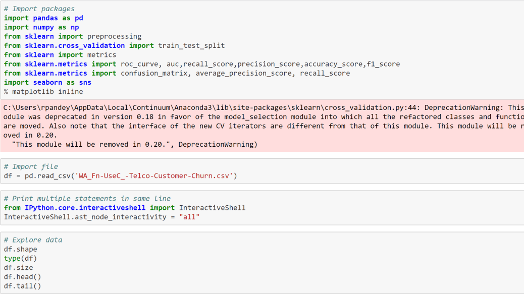
Converting categorical variables into numerical dummy coded variable is generally a requirement in machine learning libraries such as Scikit as they mostly work on numpy arrays.

In this blog, let’s look at how we can convert bunch of categorical variables into numerical dummy coded variables using four different methods-

  1. Scikit learn preprocessing LabelEncoder
  2.  Pandas getdummies
  3. Looping
  4. Mapping

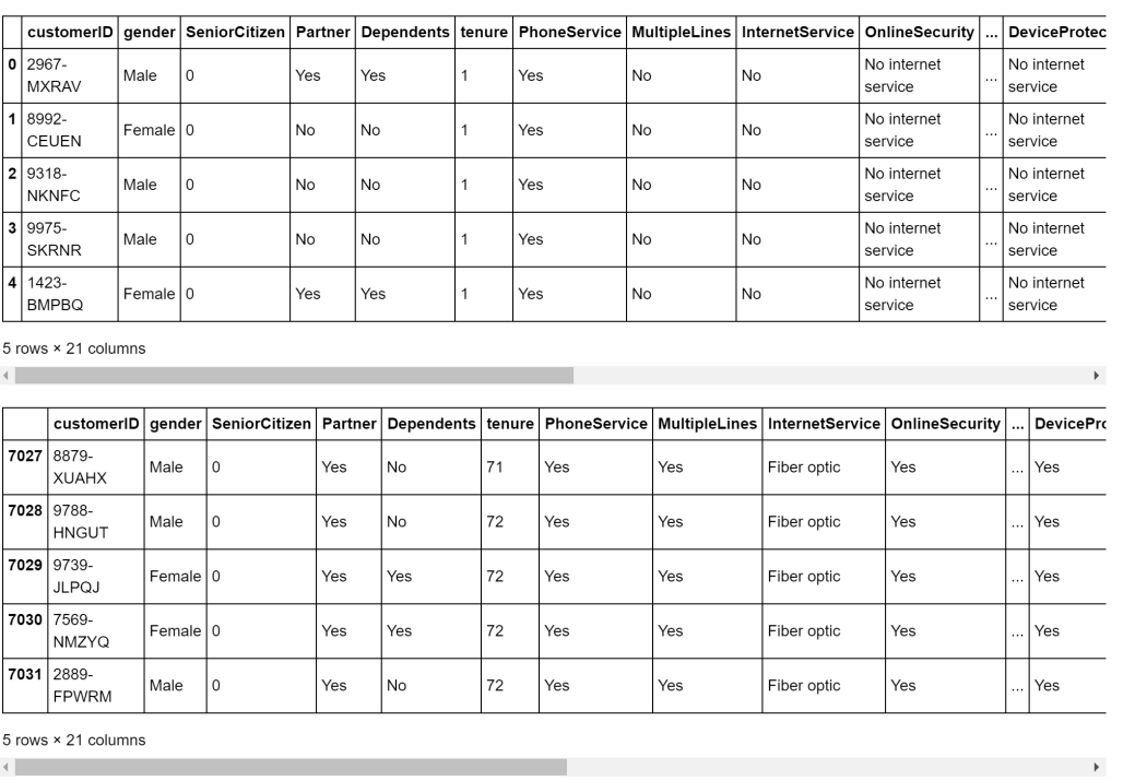
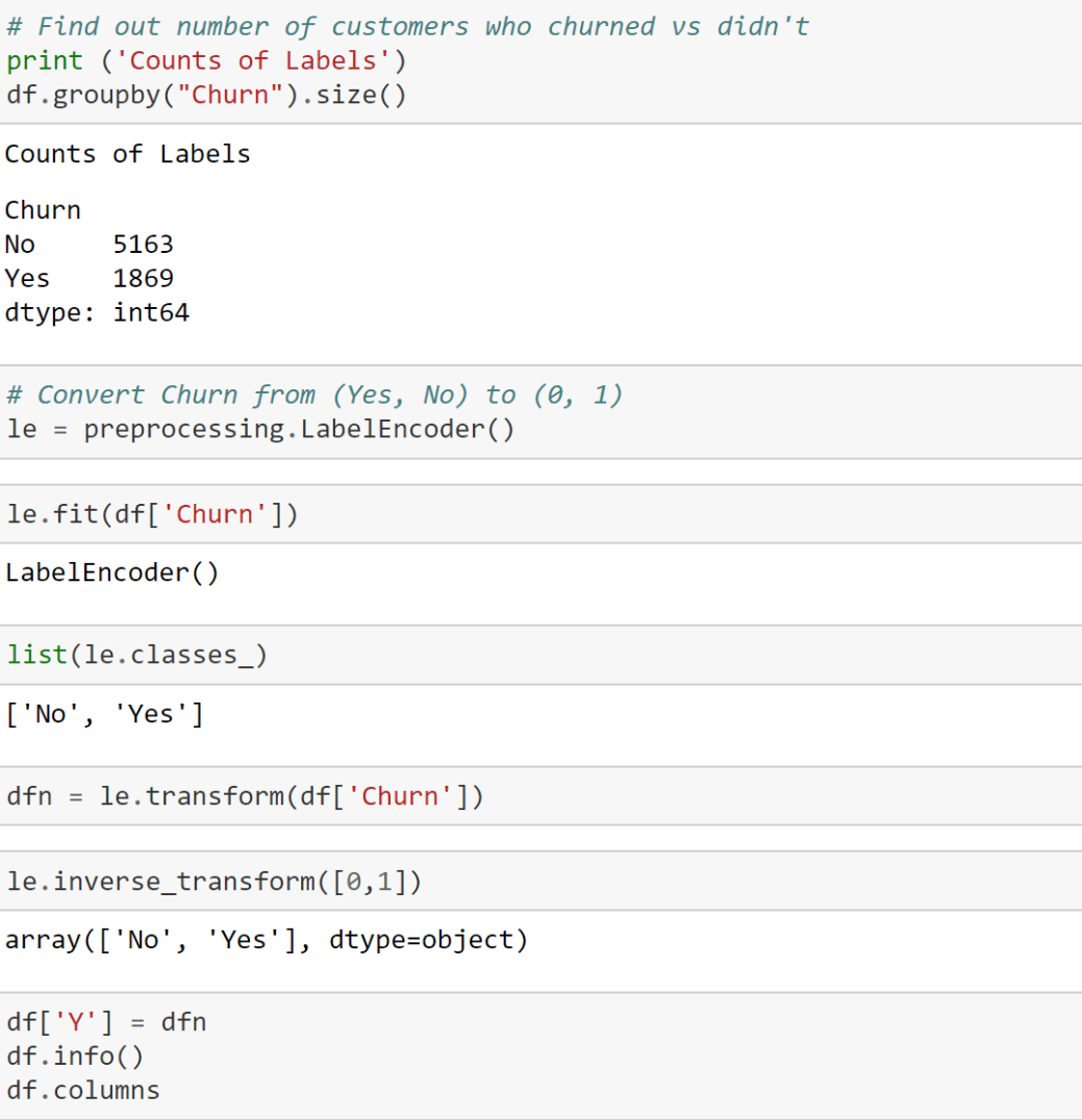
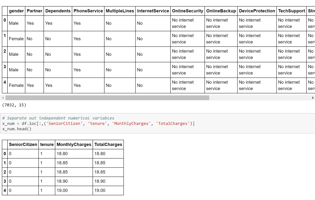
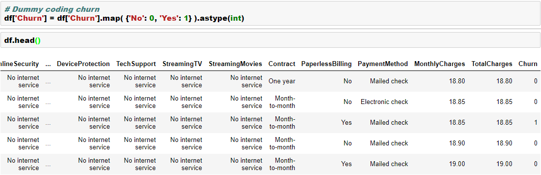
We will work with a dataset from IBM Watson blog as this has plenty of categorical variables. You can find the data here.  In this data, we are trying to build a model to predict “churn”, which has two levels “Yes” and “No”.

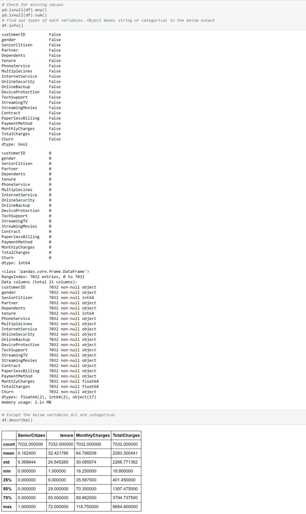
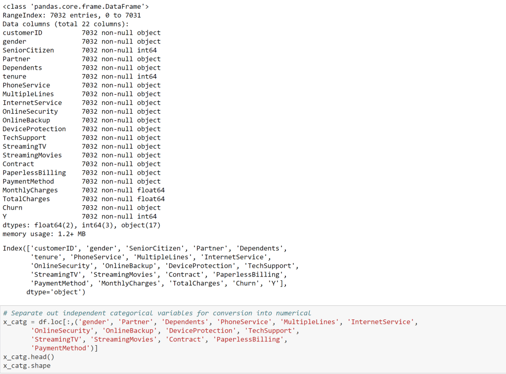
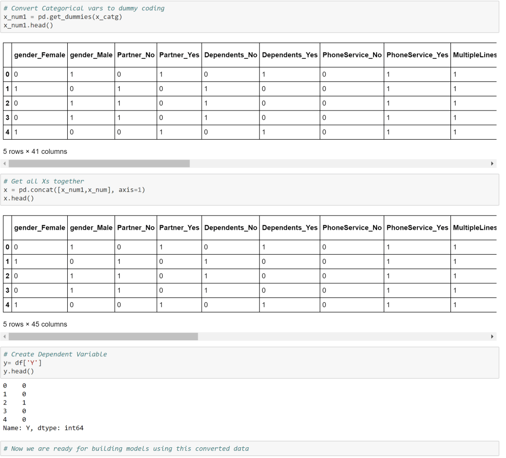
We will convert the dependent variable using Scikit LabelEncoder and the independent categorical variables using Pandas getdummies. Please note that LabelEncoder will not necessarily create additional columns, whereas the getdummies will create additional columns in the data. We will see that in the below example-

clf1clf2clf3clf4clf5clf6clf7

Here are few other ways to dummy coding-

dummy_coding1dummy_coding2dummy_coding3

Here is an excellent Kaggle Kernel for detailed feature engineering.

Cheers!

Hierarchical Clustering with Python

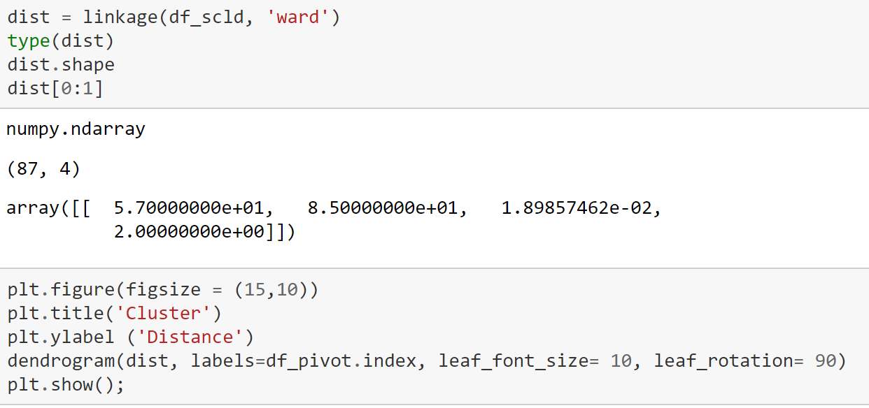
As highlighted in the article, clustering and segmentation play an instrumental role in Data Science. In this blog, we will show you how to build a Hierarchical Clustering with Python.

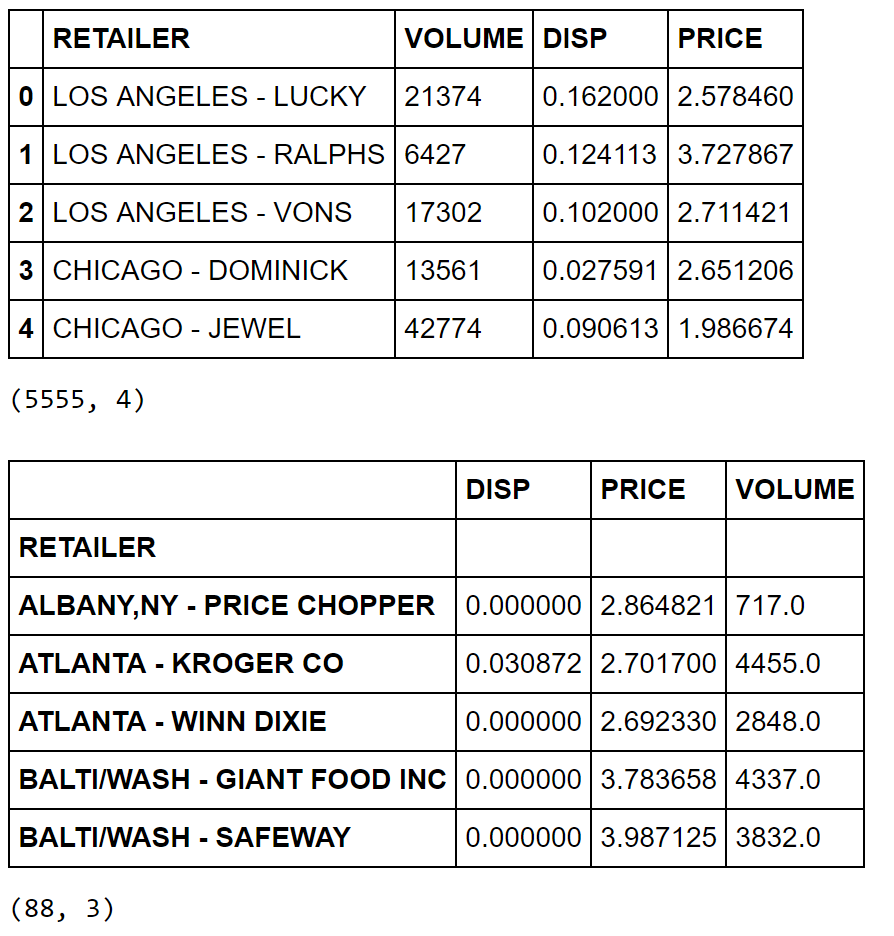
For this purpose, we will work with a R dataset called “Cheese”. Please install package called “Bayesm” in R and export this data set in csv format to be imported in Python. More on this dataset can be found here.

Let’s begin with the clustering in Python then. hclust1hclust2hclust3hclust4hclust5hclust6hclust7

hclust8

Cheers!

KMeans Clustering: Core Concepts, Assumptions, and Key Equations

Overview:
KMeans is an unsupervised machine learning algorithm used to partition data into a specified number of clusters (k). Each cluster is defined by its centroid, and the algorithm aims to minimize the distance between data points and their assigned cluster centroids.

Core Concepts:

  1. Clusters and Centroids:

    • A cluster is a group of data points that are similar to each other.
    • The centroid is the mean position of all the points in a cluster.
  2. Assignment and Update Steps:

    • Assignment: Each data point is assigned to the nearest centroid.
    • Update: The centroids are recalculated as the mean of all points assigned to each cluster.
  3. Iterative Optimization:

    • The assignment and update steps are repeated until the centroids no longer change significantly or a maximum number of iterations is reached.

Assumptions:

  • The number of clusters (k) is known and fixed in advance.
  • Clusters are roughly spherical and equally sized.
  • Data points are closer to their own cluster centroid than to others.
  • The algorithm is sensitive to the initial placement of centroids.

Key Equations:

  1. Distance Calculation:

    • The most common distance metric is Euclidean distance.
    • For a data point x and centroid c:
      Distance = sqrt( (x1 – c1)^2 + (x2 – c2)^2 + … + (xn – cn)^2 )
  2. Centroid Update:

    • For each cluster, the new centroid is the mean of all points assigned to that cluster.
    • Centroid for cluster j:
      cj = (1 / Nj) * sum(xi)
      where Nj is the number of points in cluster j, and xi are the points in cluster j.
  3. Objective Function (Inertia):

    • KMeans minimizes the sum of squared distances (inertia) between each point and its assigned centroid.
    • Inertia = sum over all clusters j [ sum over all points i in cluster j (distance(xi, cj))^2 ]

Algorithm Steps:

  1. Choose k initial centroids (randomly or using a method like k-means++).
  2. Assign each data point to the nearest centroid.
  3. Recalculate centroids as the mean of assigned points.
  4. Repeat steps 2 and 3 until centroids stabilize.

Limitations:

  • Sensitive to outliers and noise.
  • May converge to a local minimum (results can vary with different initializations).
  • Not suitable for clusters with non-spherical shapes or very different sizes.

Applications:

  • Market segmentation
  • Image compression
  • Document clustering
  • Anomaly detection

# Simple KMeans Clustering Example
import numpy as np
import matplotlib.pyplot as plt
from sklearn.datasets import make_blobs
from sklearn.cluster import KMeans
from sklearn.metrics import silhouette_score

# Generate synthetic data
X, y_true = make_blobs(n_samples=300, centers=4, cluster_std=0.60, random_state=42)

# Elbow method to find optimal k
inertia = []
k_range = range(1, 11)
for k in k_range:
    kmeans = KMeans(n_clusters=k, random_state=42)
    kmeans.fit(X)
    inertia.append(kmeans.inertia_)
plt.figure(figsize=(6,4))
plt.plot(k_range, inertia, 'bo-')
plt.axvline(x=4, color='red', linestyle='--', label='Optimal k=4')
plt.xlabel('Number of clusters (k)')
plt.ylabel('Inertia')
plt.title('Elbow Method for Optimal k')
plt.legend()
plt.grid(True)
plt.show()

# Fit KMeans with optimal k (choose visually, e.g., k=4)
k_opt = 4
kmeans = KMeans(n_clusters=k_opt, random_state=42)
labels = kmeans.fit_predict(X)

# Plot clusters
plt.figure(figsize=(7,5))
plt.scatter(X[:, 0], X[:, 1], c=labels, cmap='viridis', s=50)
plt.scatter(kmeans.cluster_centers_[:, 0], kmeans.cluster_centers_[:, 1], c='red', s=200, alpha=0.75, marker='X', label='Centers')
plt.title(f'KMeans Clustering (k={k_opt})')
plt.xlabel('Feature 1')
plt.ylabel('Feature 2')
plt.legend()
plt.show()

# Silhouette score
score = silhouette_score(X, labels)
print(f'Silhouette Score (k={k_opt}): {score:.3f}')

Silhouette Score (k=4): 0.876

# KMeans Clustering on Iris Dataset
import numpy as np
import matplotlib.pyplot as plt
from sklearn.datasets import load_iris
from sklearn.cluster import KMeans
from sklearn.metrics import silhouette_score
import pandas as pd

# Load Iris data
iris = load_iris()
X = iris.data

# Elbow method to find optimal k
inertia = []
k_range = range(1, 11)
for k in k_range:
    kmeans = KMeans(n_clusters=k, random_state=42)
    kmeans.fit(X)
    inertia.append(kmeans.inertia_)
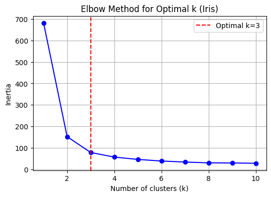
k_opt = 3  # Set optimal k explicitly for Iris data
plt.figure(figsize=(6,4))
plt.plot(k_range, inertia, 'bo-')
plt.axvline(x=k_opt, color='red', linestyle='--', label='Optimal k=3')
plt.xlabel('Number of clusters (k)')
plt.ylabel('Inertia')
plt.title('Elbow Method for Optimal k (Iris)')
plt.legend()
plt.grid(True)
plt.show()

# Fit KMeans with optimal k (choose visually, e.g., k=3)
kmeans = KMeans(n_clusters=k_opt, random_state=42)
labels = kmeans.fit_predict(X)

# Plot clusters (using first two features for visualization)
plt.figure(figsize=(7,5))
plt.scatter(X[:, 0], X[:, 1], c=labels, cmap='viridis', s=50)
plt.scatter(kmeans.cluster_centers_[:, 0], kmeans.cluster_centers_[:, 1], c='red', s=200, alpha=0.75, marker='X', label='Centers')
plt.title(f'Iris KMeans Clustering (k={k_opt})')
plt.xlabel(iris.feature_names[0])
plt.ylabel(iris.feature_names[1])
plt.legend()
plt.show()

# Plot clusters (using petal length and petal width for visualization)
plt.figure(figsize=(7,5))
plt.scatter(X[:, 2], X[:, 3], c=labels, cmap='viridis', s=50)
plt.scatter(kmeans.cluster_centers_[:, 2], kmeans.cluster_centers_[:, 3], c='red', s=200, alpha=0.75, marker='X', label='Centers')
plt.title(f'Iris KMeans Clustering (k={k_opt}) - Petal Length vs Petal Width')
plt.xlabel(iris.feature_names[2])
plt.ylabel(iris.feature_names[3])
plt.legend()
plt.show()

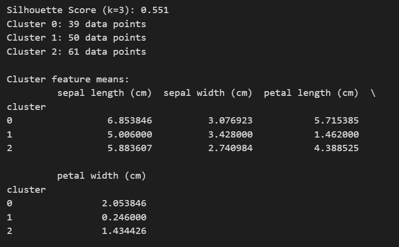
# Silhouette score
score = silhouette_score(X, labels)
print(f'Silhouette Score (k={k_opt}): {score:.3f}')

# Number of observations in each cluster
unique, counts = np.unique(labels, return_counts=True)
for i, count in zip(unique, counts):
    print(f"Cluster {i}: {count} data points")

# Descriptive summary of each cluster (mean feature values)
df = pd.DataFrame(X, columns=iris.feature_names)
df['cluster'] = labels
print("\nCluster feature means:")
print(df.groupby('cluster').mean())

Cheers!

Python Machine Learning Linear Regression with Scikit- learn

What is a “Linear Regression”-

Linear regression is one of the most powerful and yet very simple machine learning algorithm. Linear regression is used for cases where the relationship between the dependent and one or more of the independent variables is supposed to be linearly correlated in the following fashion-

Y = b0 + b1*X1 + b2*X2 + b3*X3 + …..

Here Y is the dependent variable and X1, X2, X3 etc are independent variables. The purpose of building a linear regression model is to estimate the coefficients b0, b1, b2 et cetera that provides the least error rate in the prediction. More on the error will be discussed later in this article.

In the above equation, b0 is the intercept, b1 is the coefficient for variable X1, b2 is the coefficient for the variable X2 and so on…

What is a “Simple Linear Regression” and “ Multiple Linear Regression”?

When we have only one independent variable, resulting regression is called a “Simple Linear Regression” when we have 2 or more independent variables the resulting regression is called “Multiple Linear Regression”

What are the requirements for the dependent and independent variables in the regression analysis?

The dependent variable in linear regression is generally Numerical and Continuous such as sales in dollars, gdp, unemployment rate, pollution level, amount of rainfall etc. On the other hand, the independent variables can be either numeric or categorical. However, please note that the categorical variables will need to be dummy coded before we can use these variables for building a regression model in the sklearn library of Python.

What are some of the real world usage of linear regression?

As we discussed earlier, this is one of the most commonly used algorithm in ML. Some of the use cases are listed below-

Example 1-

Predict sales amount of a car company as a function of the # of models, new models, price, discount,GDP, interest rate, unemployment rate, competitive prices etc.

Example 2-

Predict weight gain/loss of a person as a function of calories intake, junk food, genetics, exercise time and intensity, sleep, festival time, diet plans, medicines etc.

Example 3-

Predict house prices as a function of sqft, # of rooms, interest rate, parking, pollution level, distance from city center, population mix etc.

Example 4-

Predict GDP growth rate as a function of inflation, unemployment rate, investment, new business, weather pattern, resources, population

How do we evaluate linear regression model’s performance? 

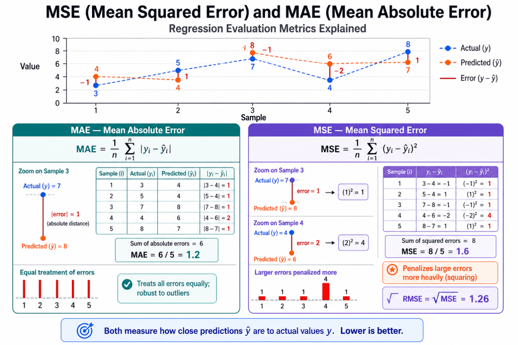
There are many metrics that can be used to evaluate a linear regression model’s performance and choose the best model.  Some of the most commonly used metrics are-

Mean Square Error (MSE)- This is an error and lower the amount the better it is. It is defined using the below formula


R Square– This is called coefficient of determination and provides a gauge of model’s explaining power. For example, for a linear regression model with a RSquare of 0.70 or 70% would imply that 70% of the variation in the dependent variable can be explained by the model that has been built.

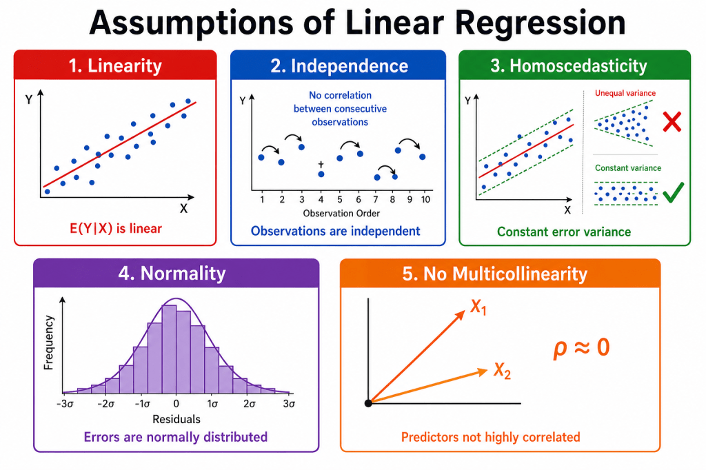
Assumptions of Linear Regression

The five assumptions

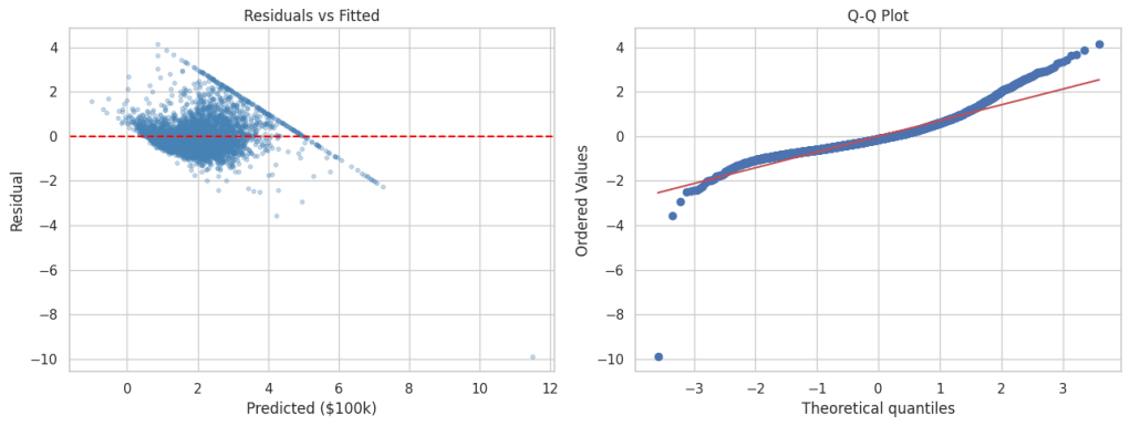
1. Linearity — E(Y|X) should follow a straight line, not a curve. Check with scatter plots and residual vs. fitted plots. Fix with transforms, polynomial terms, or nonlinear models.

2. Independence — Errors should not correlate across observations (common in time series or repeated measures). Check with Durbin–Watson or residuals vs. order. Fix with GLS, mixed models, or cluster-robust standard errors.

3. Homoscedasticity — Residual spread should stay constant across X. A funnel shape in the residual plot is a red flag. Fix with robust standard errors, WLS, or log transforms.

4. Normality  — Residuals should be roughly bell-shaped. Matters most for small samples; large samples are often more forgiving. Check with Q–Q plots.

5. No multicollinearity — Predictors should not be almost redundant. High VIF can make individual coefficients unstable even when overall prediction is fine. Fix by dropping or combining predictors, or using ridge regression.

How do we build a linear regression model in Python?

In this exercise, we will build a linear regression model on Boston housing data set which is an inbuilt data in the scikit-learn library of Python. However, before we go down the path of building a model, let’s talk about some of the basic steps in any machine learning model in Python

In most cases, any of the machine learning algorithm in sklearn library will follow the following steps-

  • Split original data into features and label. In other words,  create dependent variable and set of independent variables in two different arrays separately. Please note this requirement exists only for the supervised learning ( where a dependent variable is present). For unsupervised learning, we don’t have a dependent variable and hence there is no need to split the data into features and label
  • Scale or Normalize the features and label data. Please note that this is not a necessity for all algorithms and/or datasets. Also we are assuming that all the data cleaning and feature engineering  such as missing value treatment, outlier treatment, bogus values fixes and dummy coding of the categorical variables have been done before doing this step
  • Create training and test data sets from the original data. Training data set will be used for training the model whereas the test data set will be used for validating the accuracy or the prediction power of the model on a new dataset. We would need to split both the features and labels into the training and the test split.
  • Create an instance of the model object that will be used for the modelling exercise. This process is called “Instantiation”.  In simpler words, during this process we are loading the model package necessary to build a model.
  • “Fit” the model instance on the training data. During this step, the model is leveraging both the features and the label information provided in the training data to connect the features to label. Please note that we are going with all the default option during fitting of the model.  As you get more expertise you may want to play with some parameter optimization, however we are just going with the defaults for now.
  • “Predict” using the model instance on test data. During this step, the model is only using the features information to predict the label.
  • Based on the predictions generated on the test data, we generate key performance indicators of  model performance. This generally includes metrics such as Precision, Recall F score, Confusion Matrix, Accuracy, Mean Square Error (MSE), Root Mean Square Error (RMSE), Mean Absolute Error (MAE), Area Under the Curve (AUC), Mean Absolute Percentage error (MAPE) etc.
  • Once the model performance is evaluated and its deemed to be satisfactory for the purpose of the business uses, we implement the model for new unseen data

So let’s get started with building this model-

Overview

The dataset has 20,640 rows — one row per census block group in California (1990 U.S. Census). The goal is to predict median house value in a block from local demographic and housing features.

Target variable

ColumnDescription
MedHouseValMedian house value in the block group, in $100,000 units (e.g. 2.5 ≈ $250,000). Values are capped at 5.0 ($500,000).

Features (8 predictors)

ColumnDescription
MedIncMedian income in the block group
HouseAgeMedian age of houses in the block group
AveRoomsAverage number of rooms per household
AveBedrmsAverage number of bedrooms per household
PopulationTotal population in the block group
AveOccupAverage number of household members
LatitudeBlock group latitude
LongitudeBlock group longitude
import warnings
import matplotlib.pyplot as plt
import numpy as np
import pandas as pd
import seaborn as sns
from scipy import stats
from sklearn.datasets import fetch_california_housing
from sklearn.linear_model import LinearRegression
from sklearn.metrics import mean_absolute_error, mean_squared_error, r2_score
from sklearn.model_selection import train_test_split
from sklearn.preprocessing import StandardScaler
warnings.filterwarnings("ignore")
sns.set_theme(style="whitegrid")
# --- Load data & EDA ---
housing = fetch_california_housing()
df = pd.DataFrame(housing.data, columns=housing.feature_names)
df["MedHouseVal"] = housing.target
print("Shape:", df.shape)
print(df.head())
print(df.describe())
print("Missing values:\n", df.isnull().sum())
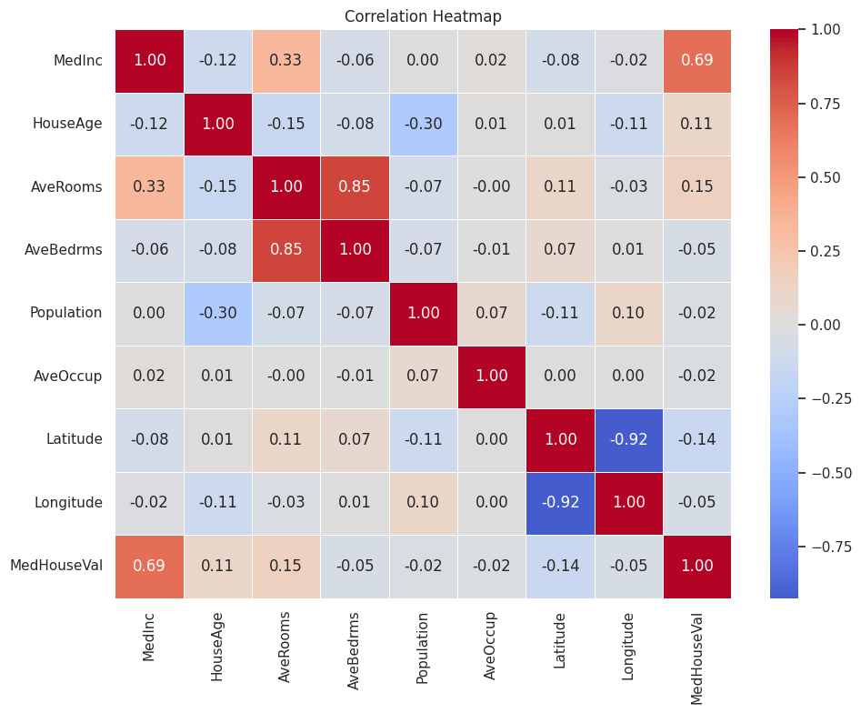
corr = df.corr()
print("\nCorrelation matrix:\n", corr.round(3))
plt.figure(figsize=(10, 8))
sns.heatmap(corr, annot=True, fmt=".2f", cmap="coolwarm", center=0, linewidths=0.5)
plt.title("Correlation Heatmap")
plt.tight_layout()
plt.show()
# --- STEP 1: features & label ---
X = df.drop("MedHouseVal", axis=1)
y = df["MedHouseVal"]
# --- STEP 2: scale ---
X_scaled = pd.DataFrame(StandardScaler().fit_transform(X), columns=X.columns)
# --- STEP 3: train/test split ---
X_train, X_test, y_train, y_test = train_test_split(
X_scaled, y, test_size=0.2, random_state=42
)
# --- STEP 4 & 5: instantiate & fit ---
model = LinearRegression()
model.fit(X_train, y_train)
print(f"\nIntercept: {model.intercept_:.4f}")
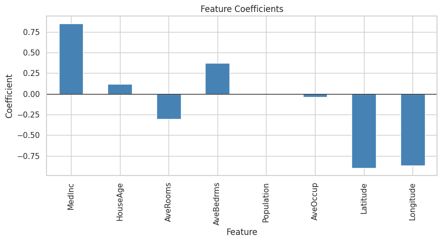
coef_df = pd.DataFrame({"Feature": X.columns, "Coefficient": model.coef_})
print(coef_df.sort_values("Coefficient", key=abs, ascending=False))
plt.figure(figsize=(9, 5))
coef_df.set_index("Feature")["Coefficient"].plot(kind="bar", color="steelblue")
plt.title("Feature Coefficients")
plt.ylabel("Coefficient")
plt.axhline(0, color="black", linewidth=0.8)
plt.tight_layout()
plt.show()
# --- STEP 6: predict & evaluate ---
y_pred = model.predict(X_test)
r2 = r2_score(y_test, y_pred)
mse = mean_squared_error(y_test, y_pred)
mae = mean_absolute_error(y_test, y_pred)
print(f"\nR² : {r2:.4f}")
print(f"MSE : {mse:.4f}")
print(f"RMSE : {np.sqrt(mse):.4f}")
print(f"MAE : {mae:.4f}")
results = pd.DataFrame({
"Actual": y_test.values,
"Predicted": y_pred,
})
results["Error"] = results["Actual"] - results["Predicted"]
results["Abs_Error"] = results["Error"].abs()
print("\nSample results:\n", results.head(10).round(4))
print("\nError summary:\n", results[["Error", "Abs_Error"]].describe().round(4))
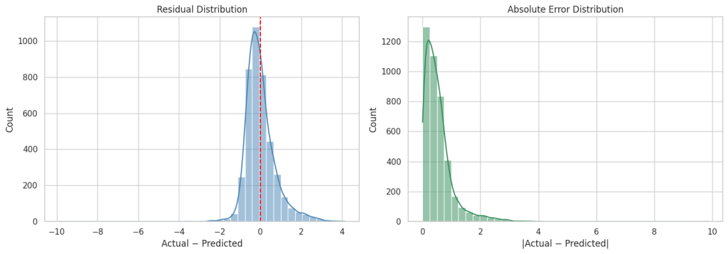
residuals = results["Error"]
abs_errors = results["Abs_Error"]
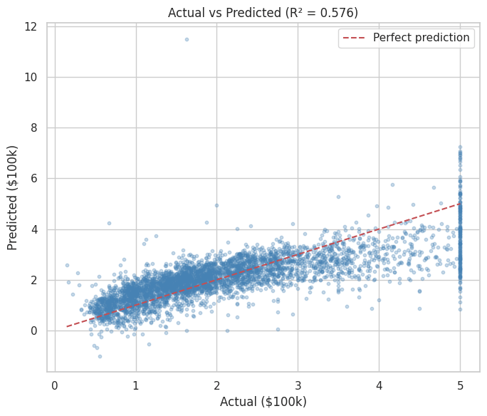
# Actual vs predicted
plt.figure(figsize=(7, 6))
plt.scatter(results["Actual"], results["Predicted"], alpha=0.3, s=10, color="steelblue")
lims = [results["Actual"].min(), results["Actual"].max()]
plt.plot(lims, lims, "r--", label="Perfect prediction")
plt.xlabel("Actual ($100k)")
plt.ylabel("Predicted ($100k)")
plt.title(f"Actual vs Predicted (R² = {r2:.3f})")
plt.legend()
plt.tight_layout()
plt.show()
# Error distributions
fig, axes = plt.subplots(1, 2, figsize=(14, 5))
sns.histplot(residuals, bins=40, kde=True, ax=axes[0], color="steelblue")
axes[0].axvline(0, color="red", linestyle="--")
axes[0].set_title("Residual Distribution")
axes[0].set_xlabel("Actual − Predicted")
sns.histplot(abs_errors, bins=40, kde=True, ax=axes[1], color="seagreen")
axes[1].set_title("Absolute Error Distribution")
axes[1].set_xlabel("|Actual − Predicted|")
plt.tight_layout()
plt.show()
# Residuals vs fitted & Q-Q plot
fig, axes = plt.subplots(1, 2, figsize=(13, 5))
axes[0].scatter(results["Predicted"], residuals, alpha=0.3, s=10, color="steelblue")
axes[0].axhline(0, color="red", linestyle="--")
axes[0].set_xlabel("Predicted ($100k)")
axes[0].set_ylabel("Residual")
axes[0].set_title("Residuals vs Fitted")
stats.probplot(residuals, dist="norm", plot=axes[1])
axes[1].set_title("Q-Q Plot")
plt.tight_layout(
plt.show()

Output from the above code-

Shape: (20640, 9)
   MedInc  HouseAge  AveRooms  AveBedrms  Population  AveOccup  Latitude  Longitude  MedHouseVal
0  8.3252      41.0  6.984127   1.023810       322.0  2.555556     37.88    -122.23        4.526
1  8.3014      21.0  6.238137   0.971880      2401.0  2.109842     37.86    -122.22        3.585
2  7.2574      52.0  8.288136   1.073446       496.0  2.802260     37.85    -122.24        3.521
3  5.6431      52.0  5.817352   1.073059       558.0  2.547945     37.85    -122.25        3.413
4  3.8462      52.0  6.281853   1.081081       565.0  2.181467     37.85    -122.25        3.422
             MedInc      HouseAge      AveRooms     AveBedrms    Population      AveOccup      Latitude     Longitude  \
count  20640.000000  20640.000000  20640.000000  20640.000000  20640.000000  20640.000000  20640.000000  20640.000000   
mean       3.870671     28.639486      5.429000      1.096675   1425.476744      3.070655     35.631861   -119.569704   
std        1.899822     12.585558      2.474173      0.473911   1132.462122     10.386050      2.135952      2.003532   
min        0.499900      1.000000      0.846154      0.333333      3.000000      0.692308     32.540000   -124.350000   
25%        2.563400     18.000000      4.440716      1.006079    787.000000      2.429741     33.930000   -121.800000   
50%        3.534800     29.000000      5.229129      1.048780   1166.000000      2.818116     34.260000   -118.490000   
75%        4.743250     37.000000      6.052381      1.099526   1725.000000      3.282261     37.710000   -118.010000   
max       15.000100     52.000000    141.909091     34.066667  35682.000000   1243.333333     41.950000   -114.310000   

        MedHouseVal  
count  20640.000000  
mean       2.068558  
std        1.153956  
min        0.149990  
25%        1.196000  
50%        1.797000  
75%        2.647250  
max        5.000010  
Missing values:
 MedInc         0
HouseAge       0
AveRooms       0
AveBedrms      0
Population     0
AveOccup       0
Latitude       0
Longitude      0
MedHouseVal    0
dtype: int64

Correlation matrix:
              MedInc  HouseAge  AveRooms  AveBedrms  Population  AveOccup  Latitude  Longitude  MedHouseVal
MedInc        1.000    -0.119     0.327     -0.062       0.005     0.019    -0.080     -0.015        0.688
HouseAge     -0.119     1.000    -0.153     -0.078      -0.296     0.013     0.011     -0.108        0.106
AveRooms      0.327    -0.153     1.000      0.848      -0.072    -0.005     0.106     -0.028        0.152
AveBedrms    -0.062    -0.078     0.848      1.000      -0.066    -0.006     0.070      0.013       -0.047
Population    0.005    -0.296    -0.072     -0.066       1.000     0.070    -0.109      0.100       -0.025
AveOccup      0.019     0.013    -0.005     -0.006       0.070     1.000     0.002      0.002       -0.024
Latitude     -0.080     0.011     0.106      0.070      -0.109     0.002     1.000     -0.925       -0.144
Longitude    -0.015    -0.108    -0.028      0.013       0.100     0.002    -0.925      1.000       -0.046
MedHouseVal   0.688     0.106     0.152     -0.047      -0.025    -0.024    -0.144     -0.046        1.000
Intercept: 2.0679
      Feature  Coefficient
6    Latitude    -0.896635
7   Longitude    -0.868927
0      MedInc     0.852382
3   AveBedrms     0.371132
2    AveRooms    -0.305116
1    HouseAge     0.122382
5    AveOccup    -0.036624
4  Population    -0.002298
R²   : 0.5758
MSE  : 0.5559
RMSE : 0.7456
MAE  : 0.5332

Sample results:
    Actual  Predicted   Error  Abs_Error
0   0.477     0.7191 -0.2421     0.2421
1   0.458     1.7640 -1.3060     1.3060
2   5.000     2.7097  2.2904     2.2904
3   2.186     2.8389 -0.6529     0.6529
4   2.780     2.6047  0.1753     0.1753
5   1.587     2.0118 -0.4248     0.4248
6   1.982     2.6455 -0.6635     0.6635
7   1.575     2.1688 -0.5938     0.5938
8   3.400     2.7407  0.6593     0.6593
9   4.466     3.9156  0.5504     0.5504

Error summary:
            Error  Abs_Error
count  4128.0000  4128.0000
mean      0.0035     0.5332
std       0.7457     0.5212
min      -9.8753     0.0001
25%      -0.4609     0.1968
50%      -0.1224     0.4102
75%       0.3124     0.6886
max       4.1484     9.8753


As you can see from the above metrics that overall this plain vanilla regression model is doing a decent job. However, it can be significantly improved upon by either doing feature engineering such as binning, multicollinearity and heteroscedasticity fixes etc. or by leveraging more robust techniques such as Elastic Net, Ridge Regression or SGD Regression, Non Linear models.

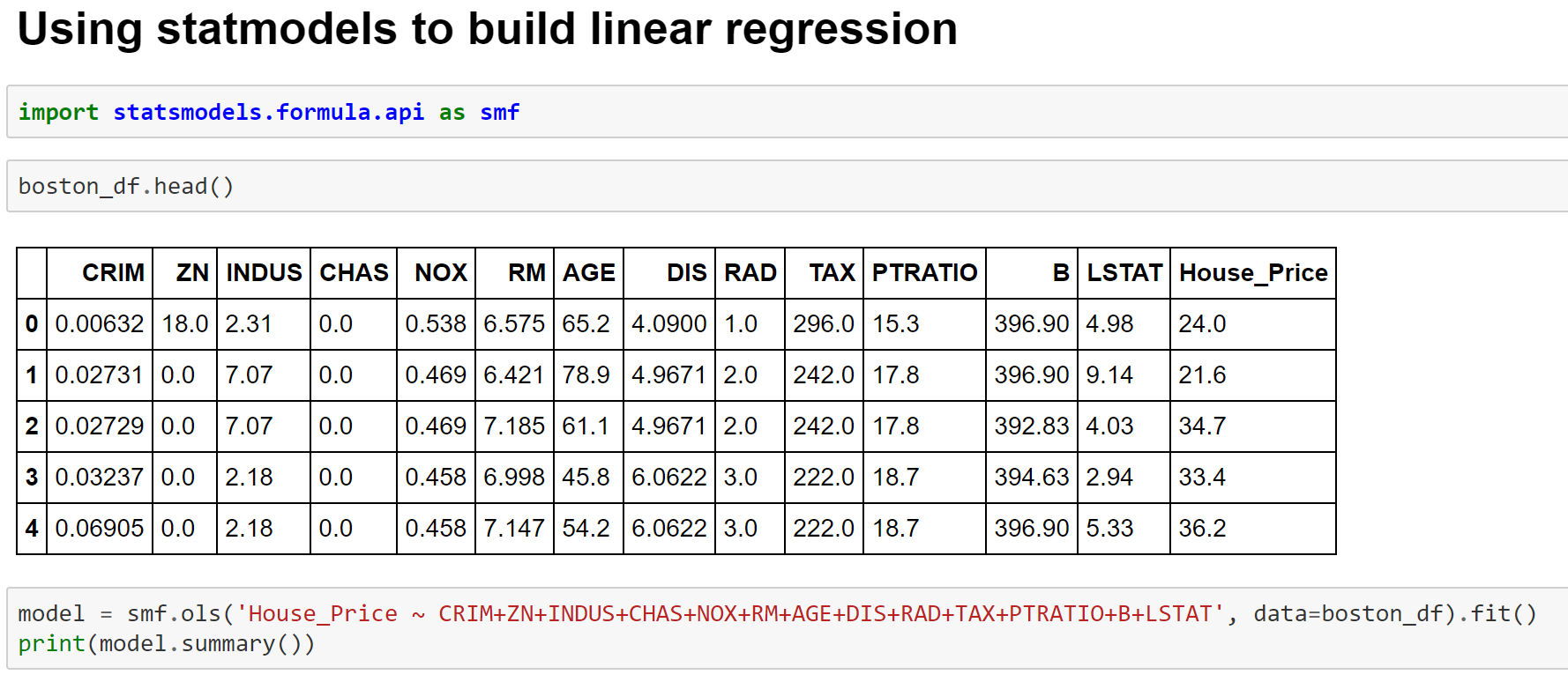
Building Linear Model using statsmodels module 

Fitting Linear Regression Model using Statmodels
Image 9- Fitting Linear Regression Model using Statmodels
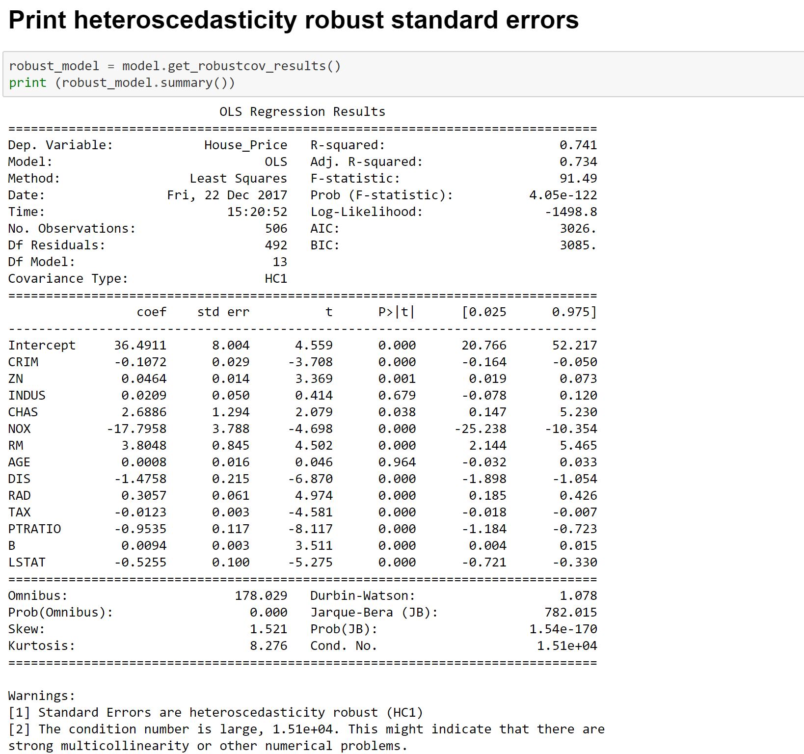
OLS Regression Output
Image 10- OLS Regression Output
itting Linear Regression Model with Significant Variables
Image 11- Fitting Linear Regression Model with Significant Variables
Heteroscedasticity Consistent Linear Regression Estimates
Image 12- Heteroscedasticity Consistent Linear Regression Estimates

More details on the metrics can be found at the below links-

Wiki

Here is a blog with excellent explanation of all metrics

Cheers!

Data Standardization or Normalization

Data standardization or normalization plays a critical role in most of the statistical analysis and modeling. Let’s spend sometime to talk about the difference between the standardization and normalization first.

Standardization is when a variable is made to follow the standard normal distribution ( mean =0  and standard deviation = 1). On the other hand, normalization is when a variable is fitted within a certain range ( generally between 0 and 1). Here are more details of the above.

Let’s now talk about why we need to do the standardization or normalization before many statistical analysis?

  1. In a multivariate analysis when variables have widely different scales, variable(s) with higher range may overshadow the other variables in analysis. For example, let’s say variable X has a range of 0-1000 and variable Y has a range of 0-10. In all likelihood, variable X will outweigh variable Y due to it’s higher range. However, if we standardize or normalize the variable, then we can overcome this issue.
  2. Any algorithms which are based on distance computations such as clustering, k nearest neigbour ( KNN), principal component ( PCA) will be greatly affected if you don’t normalize the data
  3. Neural networks and deep learning networks also need the variables to be normalized for converging faster and giving more accurate results
  4. Multivariate models may become more stable and the coefficients more reliable if you normalize the data
  5. It provides immunity from the problem of outliers

Let’s look at a Python example on how we can normalize data-

# MinMaxScaler on California Housing — before vs after
# Formula: x_scaled = (x - min) / (max - min) -> values land in [0, 1]
# In Jupyter: add `%matplotlib inline` at the top for inline charts.
import warnings
import matplotlib.pyplot as plt
import pandas as pd
import seaborn as sns
from sklearn.datasets import fetch_california_housing
from sklearn.preprocessing import MinMaxScaler
warnings.filterwarnings("ignore")
sns.set_theme(style="whitegrid")
# 1. Load features
housing = fetch_california_housing()
X = pd.DataFrame(housing.data, columns=housing.feature_names)
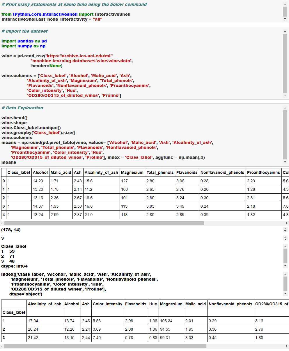
print("BEFORE MinMaxScaler (original values):\n")
print(X.head().round(3))
print("\n", X.describe().round(3))
# 2. Fit MinMaxScaler and transform
scaler = MinMaxScaler()
X_scaled = pd.DataFrame(
scaler.fit_transform(X),
columns=X.columns,
)
print("\n" + "=" * 50)
print("AFTER MinMaxScaler (scaled to [0, 1]):\n")
print(X_scaled.head().round(3))
print("\n", X_scaled.describe().round(3))
# 3. Worked example — one feature, first 5 rows
feature = "MedInc"
lo = scaler.data_min_[X.columns.get_loc(feature)]
hi = scaler.data_max_[X.columns.get_loc(feature)]
example = pd.DataFrame({
"raw": X[feature].head(),
"min": lo,
"max": hi,
})
example["scaled = (raw - min) / (max - min)"] = (
(example["raw"] - example["min"]) / (example["max"] - example["min"])
).round(3)
example["sklearn output"] = X_scaled[feature].head().round(3).values
print("\n" + "=" * 50)
print(f"How scaling works for {feature}:\n")
print(example.to_string())
# 4. Quick before / after summary
print("\n" + "=" * 50)
print("Before vs after (min and max per feature):\n")
comparison = pd.DataFrame({
"before_min": X.min(),
"before_max": X.max(),
"after_min": X_scaled.min(),
"after_max": X_scaled.max(),
}).round(3)
print(comparison.to_string())
# 5. Plots
fig, axes = plt.subplots(1, 2, figsize=(12, 5))
sns.boxplot(data=X, ax=axes[0], color="steelblue", fliersize=2)
axes[0].set_title("Before scaling")
axes[0].set_xticklabels(axes[0].get_xticklabels(), rotation=45, ha="right")
sns.boxplot(data=X_scaled, ax=axes[1], color="darkorange", fliersize=2)
axes[1].set_title("After MinMaxScaler [0, 1]")
axes[1].set_xticklabels(axes[1].get_xticklabels(), rotation=45, ha="right")
plt.suptitle("California Housing — all features", y=1.02)
plt.tight_layout()
plt.show()
fig, axes = plt.subplots(1, 2, figsize=(10, 4))
sns.histplot(X[feature], bins=40, kde=True, ax=axes[0], color="steelblue")
axes[0].set_title(f"Before — {feature}")
axes[0].set_xlabel(feature)
sns.histplot(X_scaled[feature], bins=40, kde=True, ax=axes[1], color="darkorange")
axes[1].set_title(f"After — {feature}")
axes[1].set_xlabel(f"{feature} (scaled)")
plt.tight_layout()
plt.show()
print("\nTakeaway: every feature is rescaled to the same [0, 1] range.")
print(" x_scaled = (x - column_min) / (column_max - column_min)")
BEFORE MinMaxScaler (original values):

   MedInc  HouseAge  AveRooms  AveBedrms  Population  AveOccup  Latitude  \
0   8.325      41.0     6.984      1.024       322.0     2.556     37.88   
1   8.301      21.0     6.238      0.972      2401.0     2.110     37.86   
2   7.257      52.0     8.288      1.073       496.0     2.802     37.85   
3   5.643      52.0     5.817      1.073       558.0     2.548     37.85   
4   3.846      52.0     6.282      1.081       565.0     2.181     37.85   

   Longitude  
0    -122.23  
1    -122.22  
2    -122.24  
3    -122.25  
4    -122.25  

           MedInc   HouseAge   AveRooms  AveBedrms  Population   AveOccup  \
count  20640.000  20640.000  20640.000  20640.000   20640.000  20640.000   
mean       3.871     28.639      5.429      1.097    1425.477      3.071   
std        1.900     12.586      2.474      0.474    1132.462     10.386   
min        0.500      1.000      0.846      0.333       3.000      0.692   
25%        2.563     18.000      4.441      1.006     787.000      2.430   
50%        3.535     29.000      5.229      1.049    1166.000      2.818   
75%        4.743     37.000      6.052      1.100    1725.000      3.282   
max       15.000     52.000    141.909     34.067   35682.000   1243.333   

        Latitude  Longitude  
count  20640.000  20640.000  
mean      35.632   -119.570  
std        2.136      2.004  
min       32.540   -124.350  
25%       33.930   -121.800  
50%       34.260   -118.490  
75%       37.710   -118.010  
max       41.950   -114.310  

==================================================
AFTER MinMaxScaler (scaled to [0, 1]):

   MedInc  HouseAge  AveRooms  AveBedrms  Population  AveOccup  Latitude  \
0   0.540     0.784     0.044      0.020       0.009     0.001     0.567   
1   0.538     0.392     0.038      0.019       0.067     0.001     0.565   
2   0.466     1.000     0.053      0.022       0.014     0.002     0.564   
3   0.355     1.000     0.035      0.022       0.016     0.001     0.564   
4   0.231     1.000     0.039      0.022       0.016     0.001     0.564   

   Longitude  
0      0.211  
1      0.212  
2      0.210  
3      0.209  
4      0.209  

           MedInc   HouseAge   AveRooms  AveBedrms  Population   AveOccup  \
count  20640.000  20640.000  20640.000  20640.000   20640.000  20640.000   
mean       0.232      0.542      0.032      0.023       0.040      0.002   
std        0.131      0.247      0.018      0.014       0.032      0.008   
min        0.000      0.000      0.000      0.000       0.000      0.000   
25%        0.142      0.333      0.025      0.020       0.022      0.001   
50%        0.209      0.549      0.031      0.021       0.033      0.002   
75%        0.293      0.706      0.037      0.023       0.048      0.002   
max        1.000      1.000      1.000      1.000       1.000      1.000   

        Latitude  Longitude  
count  20640.000  20640.000  
mean       0.329      0.476  
std        0.227      0.200  
min        0.000      0.000  
25%        0.148      0.254  
50%        0.183      0.584  
75%        0.549      0.631  
max        1.000      1.000  

==================================================
How scaling works for MedInc:

      raw     min      max  scaled = (raw - min) / (max - min)  sklearn output
0  8.3252  0.4999  15.0001                               0.540           0.540
1  8.3014  0.4999  15.0001                               0.538           0.538
2  7.2574  0.4999  15.0001                               0.466           0.466
3  5.6431  0.4999  15.0001                               0.355           0.355
4  3.8462  0.4999  15.0001                               0.231           0.231

==================================================
Before vs after (min and max per feature):

            before_min  before_max  after_min  after_max
MedInc           0.500      15.000        0.0        1.0
HouseAge         1.000      52.000        0.0        1.0
AveRooms         0.846     141.909        0.0        1.0
AveBedrms        0.333      34.067        0.0        1.0
Population       3.000   35682.000        0.0        1.0
AveOccup         0.692    1243.333        0.0        1.0
Latitude        32.540      41.950        0.0        1.0
Longitude     -124.350    -114.310        0.0        1.0
Takeaway: every feature is rescaled to the same [0, 1] range.
  x_scaled = (x - column_min) / (column_max - column_min)

Cheers!

Basic Statistics and Data Visualization

Doing exploratory, diagnostic and descriptive statistics is the first and very crucial part of any data analytics project.

Here are some more details on each of the steps involved in Exploratory Data Analysis ( EDA)

Let’s now look at examples on how to accomplish these tasks in Python.

You can find all the inbuilt datasets in the seaborn library using the below command-

seaborn.get_dataset_names()

The following datasets are available-

[‘anscombe’,

‘attention’,

‘brain_networks’,

‘car_crashes’,

‘diamonds’,

‘dots’,

‘exercise’,

‘flights’,

‘fmri’,

‘gammas’,

‘iris’,

‘mpg’,

‘planets’,

‘tips’,

‘titanic’]

EDA1EDA2EDA3EDA4EDA5EDA6EDA7EDA8EDA9EDA10

EDA11EDA12EDA13EDA14EDA15EDA16EDA17EDA18EDA19EDA20EDA21EDA22EDA23EDA24EDA25EDA26EDA27EDA28

Cheers!