
Decision Tree for Regression: Complete Guide and Implementation
Core Concepts and How It Works
Decision tree regression is a non-parametric supervised learning method used to predict continuous numerical values. Unlike classification trees that predict categories, regression trees predict continuous outcomes like prices, temperatures, or scores.
How Decision Trees Work for Regression
The algorithm works by recursively splitting the dataset into smaller, more homogeneous subsets based on feature values. Here’s the step-by-step process:
-
Start with the Root Node: The algorithm begins with the entire dataset at the root node
-
Find the Best Split: It evaluates all possible splits across all features to find the one that best reduces prediction error
-
Recursive Partitioning: The dataset is divided into subsets based on the chosen split, and the process repeats for each subset
-
Create Leaf Nodes: The process continues until stopping criteria are met (e.g., minimum samples per leaf, maximum depth)
-
Make Predictions: For any new data point, it follows the decision path down the tree and outputs the mean value of the training samples in the corresponding leaf node
Key Mathematical Concepts
Standard Deviation Reduction
Decision trees for regression use standard deviation reduction instead of information gain to determine the best splits. The goal is to minimize the variance within each subset after splitting.
Sum of Squared Errors (SSE)
The algorithm minimizes the Residual Sum of Squares (RSS) given by:
RSS = Sum over all regions j of Sum over observations i in region j of (yi – y_hat_Rj)^2
Where:
-
yi is the actual value for observation i
-
y_hat_Rj is the predicted value (mean) for region Rj
Mean Squared Error (MSE)
The quality of predictions is commonly evaluated using Mean Squared Error:
MSE = (1/n) * Sum of (actual_value – predicted_value)^2
Where n is the number of observations.
Core Algorithm Components
Splitting Criteria
For regression, the algorithm uses variance reduction or mean squared error reduction to evaluate splits. The feature and threshold that result in the maximum reduction in variance are chosen for each split.
Stopping Criteria
The tree stops growing when:
-
Maximum depth is reached
-
Minimum number of samples per leaf is reached
-
No further improvement in variance reduction is possible
Pruning
To prevent overfitting, cost complexity pruning is often applied, which removes branches that don’t significantly improve model performance.
Key Assumptions and Highlights
-
Non-linear Relationships: Decision trees can capture non-linear relationships between features and target variables
-
Feature Independence: The algorithm doesn’t assume independence between features
-
Local Prediction: Predictions are made locally within each leaf node using the mean of training samples
-
Greedy Algorithm: Uses a greedy approach, making the best split at each step without looking ahead
Advantages and Limitations
Advantages:
-
Easy to understand and interpret
-
Handles both numerical and categorical features
-
Requires minimal data preprocessing
-
Can capture non-linear patterns
Limitations:
-
Prone to overfitting, especially with deep trees
-
Can be unstable (small changes in data can result in different trees)
-
May create biased trees if some classes dominate
Complete Python Implementation
Here’s a comprehensive implementation that demonstrates decision tree regression with a real-world dataset:
# Import necessary libraries
import numpy as np
import pandas as pd
import matplotlib.pyplot as plt
import seaborn as sns
from sklearn.model_selection import train_test_split, cross_val_score, GridSearchCV
from sklearn.tree import DecisionTreeRegressor, plot_tree
from sklearn.metrics import mean_squared_error, r2_score, mean_absolute_error
from sklearn.preprocessing import StandardScaler
from sklearn.datasets import fetch_california_housing
import warnings
warnings.filterwarnings('ignore')
# Set random seed for reproducibility
np.random.seed(42)
print("=== Decision Tree Regression Implementation ===\n")
# 1. LOAD AND EXPLORE DATASET
print("1. Loading California Housing Dataset...")
# Load the California housing dataset - perfect for regression
california_housing = fetch_california_housing()
X = pd.DataFrame(california_housing.data, columns=california_housing.feature_names)
y = pd.Series(california_housing.target, name='MedHouseValue')
print(f"Dataset shape: {X.shape}")
print(f"Target variable range: ${y.min():.2f} - ${y.max():.2f} (in hundreds of thousands)")
print("\nFeature descriptions:")
for i, feature in enumerate(california_housing.feature_names):
print(f"- {feature}: {california_housing.DESCR.split('Attribute Information:')[1].split(':')[i+1].split('-')[0].strip()}")
# Display basic statistics
print("\nDataset Info:")
print(X.describe().round(2))
print(f"\nTarget variable statistics:")
print(y.describe().round(2))
# 2. DATA PREPROCESSING
print("\n2. Data Preprocessing...")
# Check for missing values
print(f"Missing values in features: {X.isnull().sum().sum()}")
print(f"Missing values in target: {y.isnull().sum()}")
# Feature correlation analysis
print("\nFeature correlation with target:")
correlations = X.corrwith(y).sort_values(ascending=False)
print(correlations.round(3))
# 3. TRAIN-TEST SPLIT
print("\n3. Splitting data into train and test sets...")
X_train, X_test, y_train, y_test = train_test_split(
X, y, test_size=0.2, random_state=42, shuffle=True
)
print(f"Training set size: {X_train.shape[0]} samples")
print(f"Test set size: {X_test.shape[0]} samples")
# 4. MODEL TRAINING WITH HYPERPARAMETER TUNING
print("\n4. Training Decision Tree Regressor with Hyperparameter Tuning...")
# Define hyperparameter grid for optimization
param_grid = {
'max_depth': [3, 5, 7, 10, 15, None],
'min_samples_split': [2, 5, 10, 20],
'min_samples_leaf': [1, 2, 5, 10],
'max_features': ['auto', 'sqrt', 'log2', None]
}
# Initialize the regressor
dt_regressor = DecisionTreeRegressor(random_state=42)
# Perform grid search with cross-validation
print("Performing Grid Search with 5-fold Cross Validation...")
grid_search = GridSearchCV(
estimator=dt_regressor,
param_grid=param_grid,
cv=5,
scoring='neg_mean_squared_error',
n_jobs=-1,
verbose=0
)
# Fit the grid search
grid_search.fit(X_train, y_train)
# Get the best model
best_dt = grid_search.best_estimator_
print(f"Best parameters: {grid_search.best_params_}")
print(f"Best cross-validation score (negative MSE): {grid_search.best_score_:.4f}")
# Train a simple model for comparison
simple_dt = DecisionTreeRegressor(max_depth=5, random_state=42)
simple_dt.fit(X_train, y_train)
# 5. MODEL EVALUATION
print("\n5. Model Evaluation...")
# Make predictions
y_train_pred_best = best_dt.predict(X_train)
y_test_pred_best = best_dt.predict(X_test)
y_train_pred_simple = simple_dt.predict(X_train)
y_test_pred_simple = simple_dt.predict(X_test)
# Calculate metrics for both models
def calculate_metrics(y_true, y_pred, model_name, dataset_type):
mse = mean_squared_error(y_true, y_pred)
rmse = np.sqrt(mse)
mae = mean_absolute_error(y_true, y_pred)
r2 = r2_score(y_true, y_pred)
print(f"\n{model_name} - {dataset_type} Set Metrics:")
print(f" Mean Squared Error (MSE): {mse:.4f}")
print(f" Root Mean Squared Error (RMSE): {rmse:.4f}")
print(f" Mean Absolute Error (MAE): {mae:.4f}")
print(f" R² Score: {r2:.4f}")
return mse, rmse, mae, r2
# Evaluate both models
calculate_metrics(y_train, y_train_pred_best, "Best Tuned Model", "Training")
calculate_metrics(y_test, y_test_pred_best, "Best Tuned Model", "Test")
calculate_metrics(y_train, y_train_pred_simple, "Simple Model", "Training")
calculate_metrics(y_test, y_test_pred_simple, "Simple Model", "Test")
# Cross-validation scores
cv_scores_best = cross_val_score(best_dt, X_train, y_train, cv=5, scoring='neg_mean_squared_error')
cv_scores_simple = cross_val_score(simple_dt, X_train, y_train, cv=5, scoring='neg_mean_squared_error')
print(f"\nCross-validation RMSE (Best Model): {np.sqrt(-cv_scores_best.mean()):.4f} (+/- {np.sqrt(cv_scores_best.std() * 2):.4f})")
print(f"Cross-validation RMSE (Simple Model): {np.sqrt(-cv_scores_simple.mean()):.4f} (+/- {np.sqrt(cv_scores_simple.std() * 2):.4f})")
# 6. FEATURE IMPORTANCE ANALYSIS
print("\n6. Feature Importance Analysis...")
feature_importance = pd.DataFrame({
'feature': X.columns,
'importance_best': best_dt.feature_importances_,
'importance_simple': simple_dt.feature_importances_
}).sort_values('importance_best', ascending=False)
print("Top 5 Most Important Features (Best Model):")
print(feature_importance.head())
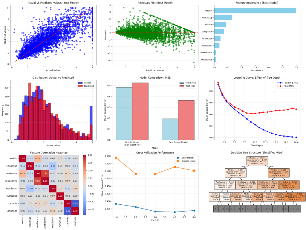
# 7. VISUALIZATIONS
print("\n7. Generating Visualizations...")
# Set up the plotting style
plt.style.use('default')
fig = plt.figure(figsize=(20, 15))
# Plot 1: Actual vs Predicted (Best Model)
plt.subplot(3, 3, 1)
plt.scatter(y_test, y_test_pred_best, alpha=0.6, color='blue', s=30)
plt.plot([y_test.min(), y_test.max()], [y_test.min(), y_test.max()], 'r--', linewidth=2)
plt.xlabel('Actual Values')
plt.ylabel('Predicted Values')
plt.title('Actual vs Predicted Values (Best Model)')
plt.grid(True, alpha=0.3)
# Plot 2: Residuals Plot (Best Model)
plt.subplot(3, 3, 2)
residuals = y_test - y_test_pred_best
plt.scatter(y_test_pred_best, residuals, alpha=0.6, color='green', s=30)
plt.axhline(y=0, color='red', linestyle='--', linewidth=2)
plt.xlabel('Predicted Values')
plt.ylabel('Residuals')
plt.title('Residuals Plot (Best Model)')
plt.grid(True, alpha=0.3)
# Plot 3: Feature Importance
plt.subplot(3, 3, 3)
plt.barh(feature_importance['feature'], feature_importance['importance_best'], color='skyblue')
plt.xlabel('Importance')
plt.title('Feature Importance (Best Model)')
plt.gca().invert_yaxis()
# Plot 4: Prediction Distribution
plt.subplot(3, 3, 4)
plt.hist(y_test, bins=30, alpha=0.7, label='Actual', color='blue', edgecolor='black')
plt.hist(y_test_pred_best, bins=30, alpha=0.7, label='Predicted', color='red', edgecolor='black')
plt.xlabel('House Value')
plt.ylabel('Frequency')
plt.title('Distribution: Actual vs Predicted')
plt.legend()
plt.grid(True, alpha=0.3)
# Plot 5: Model Comparison (MSE)
plt.subplot(3, 3, 5)
models = ['Simple Model\n(max_depth=5)', 'Best Tuned Model']
train_mse = [mean_squared_error(y_train, y_train_pred_simple), mean_squared_error(y_train, y_train_pred_best)]
test_mse = [mean_squared_error(y_test, y_test_pred_simple), mean_squared_error(y_test, y_test_pred_best)]
x = np.arange(len(models))
width = 0.35
plt.bar(x - width/2, train_mse, width, label='Train MSE', color='lightblue', edgecolor='black')
plt.bar(x + width/2, test_mse, width, label='Test MSE', color='lightcoral', edgecolor='black')
plt.xlabel('Model')
plt.ylabel('Mean Squared Error')
plt.title('Model Comparison: MSE')
plt.xticks(x, models)
plt.legend()
plt.grid(True, alpha=0.3)
# Plot 6: Learning Curve (Tree Depth)
plt.subplot(3, 3, 6)
depths = range(1, 21)
train_scores = []
test_scores = []
for depth in depths:
dt_temp = DecisionTreeRegressor(max_depth=depth, random_state=42)
dt_temp.fit(X_train, y_train)
train_scores.append(mean_squared_error(y_train, dt_temp.predict(X_train)))
test_scores.append(mean_squared_error(y_test, dt_temp.predict(X_test)))
plt.plot(depths, train_scores, 'o-', color='blue', label='Training MSE', linewidth=2)
plt.plot(depths, test_scores, 'o-', color='red', label='Test MSE', linewidth=2)
plt.xlabel('Tree Depth')
plt.ylabel('Mean Squared Error')
plt.title('Learning Curve: Effect of Tree Depth')
plt.legend()
plt.grid(True, alpha=0.3)
# Plot 7: Correlation Heatmap
plt.subplot(3, 3, 7)
correlation_matrix = X.corr()
sns.heatmap(correlation_matrix, annot=True, cmap='coolwarm', center=0, square=True, fmt='.2f')
plt.title('Feature Correlation Heatmap')
# Plot 8: Cross-validation Scores
plt.subplot(3, 3, 8)
cv_results = pd.DataFrame({
'Fold': range(1, 6),
'Best Model': -cv_scores_best,
'Simple Model': -cv_scores_simple
})
plt.plot(cv_results['Fold'], cv_results['Best Model'], 'o-', label='Best Model', linewidth=2, markersize=8)
plt.plot(cv_results['Fold'], cv_results['Simple Model'], 's-', label='Simple Model', linewidth=2, markersize=8)
plt.xlabel('CV Fold')
plt.ylabel('Mean Squared Error')
plt.title('Cross-Validation Performance')
plt.legend()
plt.grid(True, alpha=0.3)
# Plot 9: Tree Visualization (Simple Model)
plt.subplot(3, 3, 9)
plot_tree(simple_dt, max_depth=3, feature_names=X.columns, filled=True, fontsize=8)
plt.title('Decision Tree Structure (Simplified View)')
plt.tight_layout()
plt.show()
# 8. DETAILED ANALYSIS AND INSIGHTS
print("\n8. Model Analysis and Insights...")
# Analyze overfitting
train_r2_best = r2_score(y_train, y_train_pred_best)
test_r2_best = r2_score(y_test, y_test_pred_best)
train_r2_simple = r2_score(y_train, y_train_pred_simple)
test_r2_simple = r2_score(y_test, y_test_pred_simple)
print(f"\nOverfitting Analysis:")
print(f"Best Model - Train R²: {train_r2_best:.4f}, Test R²: {test_r2_best:.4f}")
print(f"Simple Model - Train R²: {train_r2_simple:.4f}, Test R²: {test_r2_simple:.4f}")
overfitting_best = train_r2_best - test_r2_best
overfitting_simple = train_r2_simple - test_r2_simple
print(f"Overfitting Gap (Best): {overfitting_best:.4f}")
print(f"Overfitting Gap (Simple): {overfitting_simple:.4f}")
# Model complexity analysis
print(f"\nModel Complexity:")
print(f"Best Model - Tree Depth: {best_dt.get_depth()}, Leaves: {best_dt.get_n_leaves()}")
print(f"Simple Model - Tree Depth: {simple_dt.get_depth()}, Leaves: {simple_dt.get_n_leaves()}")
# Feature importance insights
print(f"\nKey Insights:")
print(f"• Most important feature: {feature_importance.iloc[0]['feature']} ({feature_importance.iloc[0]['importance_best']:.3f})")
print(f"• Least important feature: {feature_importance.iloc[-1]['feature']} ({feature_importance.iloc[-1]['importance_best']:.3f})")
# Performance summary
print(f"\nFinal Model Performance Summary:")
print(f"• Best model RMSE on test set: ${np.sqrt(mean_squared_error(y_test, y_test_pred_best)):.2f} (hundreds of thousands)")
print(f"• This represents an average prediction error of ~${np.sqrt(mean_squared_error(y_test, y_test_pred_best))*100000:.0f}")
print(f"• Model explains {test_r2_best:.1%} of the variance in house prices")
print("\n=== Analysis Complete ===")
Thanks for reading!


You must be logged in to post a comment.