


Month: July 2018
Auto Regressive Integrated Moving Average (ARIMA) Time Series Forecasting

Autoregressive Integrated Moving Average (ARIMA) is one of the most popular technique for time series modeling. This is also called Box-Jenkins method, named after the statisticians who pioneered some of the latest developments on this technique.
We will focus on following broad areas-
- What is a time series? We have covered this in another article. Click here
- Explore a time series data. Please refer to the slides 2 to 7 of the below deck and Click here
- What is an ARIMA modeling
- Discuss stationarity of a time series
- Fit an ARIMA model, evaluate model’s accuracy and forecast for future
What is an ARIMA modeling-
An ARIMA model has following main components. However, not all models need to have all of the below mentioned components.
- Autoregressive (AR)
Value of a time series at time period t (yt) is a function of values of time series at previous time periods ‘p’
yt = Linear function of yt-1, yt-2,….., yt-p + error
- Integrated (I)
To make a time series stationary (discussed below), sometimes we need to difference successive observation and model that. This process is known as integration and differencing order is represented as ‘d’ in an ARIMA model.
- Moving Average (MA)
Value of a time series at time period t (yt) is a function of errors at previous time periods ‘q’
yt = Linear function of Et-1, Et-2,….., Et-q + error
Based on the combinations of the above factors, we can have following and other models-
- AR- Only autoregressives terms
- MA- Only moving averages terms
- ARMA- Both autoregressive and moving average terms
- ARIMA- Autoregressive, moving average terms and integration terms. After the differencing step, the model becomes ARMA
A general ARIMA model is represented as ARIMA(p,d,q) where p, d and q represent AR, Integrated and moving averages respectively. Whereas each of p,d and q are integers higher than or equal to zero.
Stationarity of a time series-
A time series is called stationary where it has a constant mean and variance across the time period, i.e. mean and variance don’t depend on time. It other words, it should not have any trend and dispersion in variance of the data over a period of time. This is also called white noise.
Please refer to slides 8 to 11 of the below deck for live examples of this discussion
From the plot of our air passengers time series, we can tell that the time series is not stationary. Moreover, a time series needs to be stationary or made stationary before being fed into ARIMA modeling.
Statistically, Augmented Dickey–Fuller test is used for testing the stationarity of a time series. Generally speaking the null hypothesis (H0) is that the series is “Non-Stationary” and the alternative hypothesis (Ha) is that series is “Stationary”.
If the p statistics generated from the test is less than <0.05 we can reject the null hypothesis. Otherwise, we need to accept the null hypothesis.
From the ADF test we can see that the p values is close to 0.78 and which is more than 0.05 and hence we need to accept the null hypothesis that is the series is “Non Stationary”
How do we make a time series stationary? Well, we can do it two ways-
- Manual- Transformation and Differecing etc. Let’s look at an example.
- Automated- The Integrated term (d)in the ARIMA will make it stationary. This we will do in the model fitting phase. Generally speaking we don’t require d>1 to make a time series stationary
- Auto.arima ( ) will take care of this automatically and fit the best model
Fit a model, evaluate model’s accuracy and forecast
We will use auto.arima ( ) to fit the best model and evaluate model fitment and performance using following main parameters.
Please refer to slides 12-18 of the below deck
A good time series model should have following characteristics-
- Residuals shouldn’t show any trends over time.
- Auto correlation Factors(ACF) and Partial Auto correlation Factor (PACF) shouldn’t have large values (beyond significance level)for any lags. ACF indicates correlation between the current value to all the previous values in a range. PACF is an extension of ACF, where it removes the correlation of the intermediate lags. You can read more on this here.
- Errors shouldn’t show any seasonality
- Errors should be normally distributed
- Error (MAE, MAPE, MSE etc.) should be low
- AIC, BIC should be relatively lower compared to other alternative models.
For those who would like to read more about the time series analysis in R, here is an excellent free book.
Thank you!
Holt Winters Time Series Forecasting
What is a time series?
When we track a certain variable over an interval of time (generally at an equal interval of time) the resulting process is called a time series.
Let’s Look at some examples of time series in our daily life
1. Closing price of Apple stock on a daily basis will be a time series
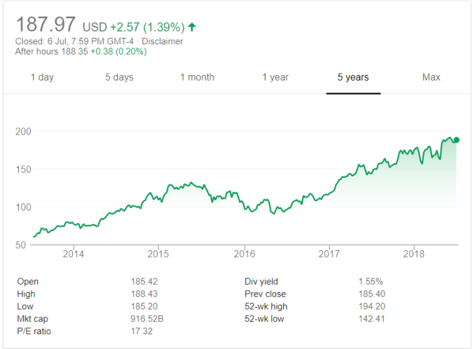
Example of Time Series- Apple Stock Price Trend Pulled from Google Finance
2. GDP of the world over last several decades so will again be a time series again-
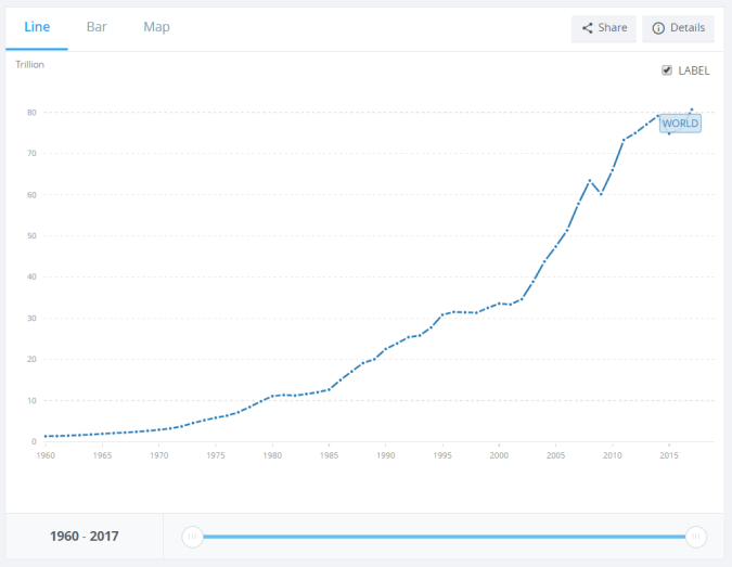
Example of Time Series- World GDP Trend Over Last Several Decades from World Bank
3. Similarly, the hourly movement of the Bitcoin prices in a day will be a time series

Example of Time Series- Hourly Bitcoin Prices from Coindesk
As you can see from the above examples, the duration of the time can vary for a time series. It can be minutes, days, hours, weeks. months, quarters, years or any other time period. However, one thing that will be common in all time series will be that a particular variable is being measured over a period of time.
What is a time series modeling?
A time series modelling is a statistical exercise where we try to achieve following two main objectives,
1. Visualize and understand the pattern of a particular time series. For example, if you are looking at the sales of an eCommerce company you would like to understand how it has performed over a period of time, which months it goes higher and lower etc.
2. By looking into the historical pattern, forecast what may happen in the future in that particular time series
What are the business usage of a time series modeling?
Time series modelling is used for a variety of different purpose. Some examples are listed below-
1. Forecast sales of an eCommerce company for the next quarter and next one year for financial planning and budgeting
2. Forecast call volume on a given day to efficiently plan resources in a call center
3. Predict trends in the future stock price movement for technical trading of that stock in a stock market
How is a time series forecasting different from a regression modeling?
One of the biggest difference between a time series and regression modeling is that a time series leverages the past value of the same variable to predict what is going to happen in the future.
On the other hand, a regression modeling such as a multiple linear regression will predict the value of a certain variable as a function of other variables
Let’s take an example to make this point more clear. If you are trying to protect the sales of an E-Commerce company as a function of what has been the sales in the past quarter this is a time series modelling
On the other hand, if you are trying to predict the sales of the same E-Commerce company as a function of other variables such as the marketing spend, price of the product and other such contributing factors, it is a regression modelling
What are the constituents of a time series?
A time series could be made up of following main parts
1. Trend- A systematic pattern of how the time series is behaving over a period of time. For example- GDP of emerging economies such as India is growing over a period of time
2. Seasonality- Peaks and troughs which happen during the same time. For example- sales of retailers in US goes higher during Thanksgiving and Black Friday
3. Random noise- As the name suggests, this is the random pattern in a time series
4. Cyclical- Cycles such as Fuel prices go low during certain time and higher at other times. Generally speaking a cycle is long in duration.
Please note that not all time series will have all these components.
Let’s look at example of the time series components. This has been done in R using the decompose function.
Additive Seasonal Model-
This model is used when the time series shows additive seasonality. For example, an eCommerce company sales in October of each year is $2MM USD higher than the base level sales regardless of what is the base level sales in that particular year. In very simplified mathematical equation it can be represented as
Observed = Trend + Seasonal + Random
Please take a look at the slide 2 and 3 of the below presentation
Multiplicative Seasonal Model-
This model is used when the time series shows multiplicative seasonality. For example, for an eCommerce company sales in October of each year is 1.2 times the base level sales in the year. If a particular year has low base level sales, the sales in October will be lower in absolute sense, however it will be 1.2x of the base level sales. In very simplified mathematical equation it can be represented as
Observed = Trend x Seasonal x Random
Please take a look a the slide 4 of the below presentation
Let’s now fit Exponential Smoothing to the above data example. Holt Winters is one of the most popular technique for doing exponential smoothing of a time series data. Moreover, we can fit both additive and multiplicative seasonal time series using HoltWinters() function in R.
There are many parameters that one can pass on this method, however one doesn’t need to pick these parameters as R will automatically pick the best settings to minimize the Square Error between the predicted and the actual values for the forecast.
The three most important parameters that one needs to pay attention to are-
alpha = Value of smoothing parameter for the base level.
beta = Value of smoothing parameter for the trend.
gamma = Value of smoothing parameter for the seasonal component.
All three of the above parameters range between 0 and 1
- If beta and gamma are both zero and alpha is non zero, this is known as Single Exponential Smoothing
- If gamma is zero but both beta and alpha are non zero, this is known as Double Exponential Smoothing with trend
- If all three of them are non zero, this is knows as Triple Exponential Smoothing or Holt Winters with trend and seasonality.
In the below example, we will let R choose the optimized parameters for us.
Additive Seasonal Holt Winters Model
Let’s fit an additive model first and compute MAE. The general form of an additive model is shown below.
yt = base + linear * t + St + Random Error
Where
yt = forecast at time period t
base = Base signal
linear = linear trend component
t= time period t
St = Additive seasonal factor
This is the model that R has fitted for us-
HoltWinters(x = fl, seasonal = “additive”)
Smoothing parameters:
alpha: 0.2479595
beta : 0.03453373
gamma: 1
Coefficients:
[,1]
a 477.827781
b 3.127627
s1 -27.457685
s2 -54.692464
s3 -20.174608
s4 12.919120
s5 18.873607
s6 75.294426
s7 152.888368
s8 134.613464
s9 33.778349
s10 -18.379060
s11 -87.772408
s12 -45.827781
See Slide # 11 on how to use the above model output to compute forecast for any given time period. However, you don’t have to do it by hand as R will do it for you. Nevertheless, good to know how to use the above model output.
Finally, let’s notice that MAE of the additive model comes out to be 9.774438
Multiplicative Seasonal Holt Winters Model
The general form of a multiplicative model is shown below-
yt = (base + linear * t )* St + Random Error
Where
yt = forecast at time period t
base = Base signal
linear = linear trend component
t= time period t
St = Additive seasonal factor
This is the model that R has fitted for us-
Call:
HoltWinters(x = fl, seasonal = “multiplicative”)
Smoothing parameters:
alpha: 0.2755925
beta : 0.03269295
gamma: 0.8707292
Coefficients:
[,1]
a 469.3232206
b 3.0215391
s1 0.9464611
s2 0.8829239
s3 0.9717369
s4 1.0304825
s5 1.0476884
s6 1.1805272
s7 1.3590778
s8 1.3331706
s9 1.1083381
s10 0.9868813
s11 0.8361333
s12 0.9209877
As you can see from the above output, the seasonality shows that demand for the air travel is the highest in July and August of each year and lowest in November.
Moreover the MAE for this model is 8.393662. Therefore, in this case a multiplicative Holt Winters seasonal model is able to provide us a better forecast compared to an additive model.
All the codes and output can be found here and in the below presentation.
Here is the forecast generated from the model-

HoltWinters Timeseries in R- Forecast for next 20 months using Multiplicative Model
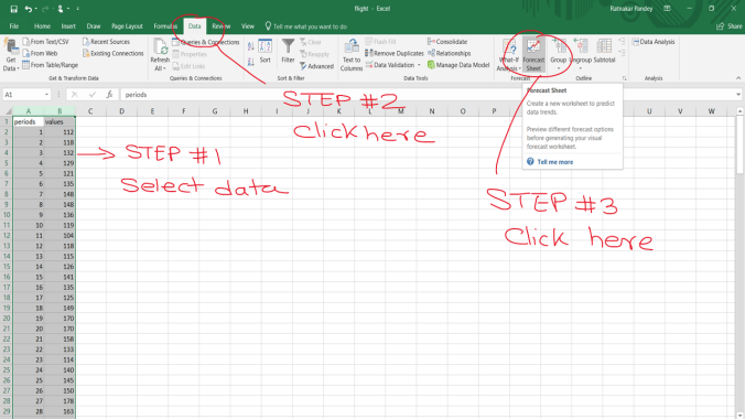
You can do the HoltWinters Forecast in Excel as well using the below simple steps-


Thank you!

You must be logged in to post a comment.