Recommendation engines or systems are all around us. Few common examples are-
- Amazon- People who buy this also buy this or who viewed this also viewed this
- Facebook- Friends recommendation
- Linkedin- Jobs that match you or network recommendation or who viewed this profile also viewed this profile
- Netflix- Movies recommendation
- Google- news recommendation, youtube videos recommendation
and so on…
The main objective of these recommendation systems is to do following-
- Customization or personalizaiton
- Cross sell
- Up sell
- Customer retention
- Address the “Long Tail” phenomenon seen in Online stores vs Brick and Mortar stores
etc..
There are three main approaches for building any recommendation system-
- Collaborative Filtering–
Users and items matrix is built. Normally this matrix is sparse, i.e. most of the cells will be empty. The goal of any recommendation system is to find similarities among the users and items and recommend items which have high probability of being liked by a user given the similarities between users and items.
Similarities between users and items can be assessed using several similarity measures such as Correlation, Cosine Similarities, Jaccard Index, Hamming Distance. The most commonly used similarity measures are Cosine Similarity and Jaccard Index in a recommendation engine
- Content Based-
This type of recommendation engine focuses on finding the characteristics, attributes, tags or features of the items and recommend other items which have some of the same features. Such as recommend another action movie to a viewer who likes action movies.
- Hybrid-
These recommendation systems combine both of the above approaches.
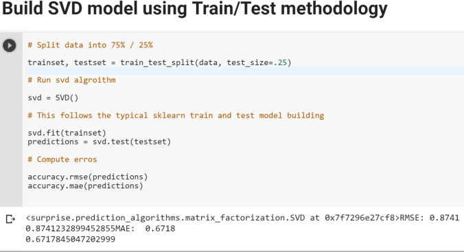
Build Recommendation System in Python using ” Scikit – Surprise”-
Now let’s switch gears and see how we can build recommendation engines in Python using a special Python library called Surprise.
This library offers all the necessary tools such as different algorithms (SVD, kNN, Matrix Factorization), in built datasets, similarity modules (Cosine, MSD, Pearson), sampling and models evaluations modules.
Here is how you can get started
- Step 1- Switch to Python 2.7 Kernel, I couldn’t make it work in 3.6 and hence needed to install 2.7 as well in my Jupyter notebook environment
- Step 2- Make sure you have Visual C++ compilers installed on your system as this package requires Cython Wheels. Here are couple of links to help you in this effort
Please note that if you don’t do the Step 2 correctly, you will get errors such as shown below – ” Failed building wheel for Scikit-surprise” or ” Microsoft Visual C++ 14 is required”

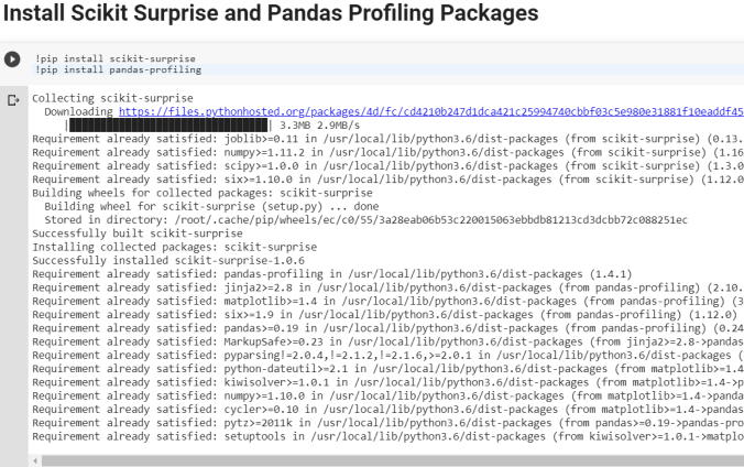
- Step 3- Install Scikit- Surprise. Please make sure that you have Numpy installed before this
pip install numpy
pip install scikit-surprise
- Step 4- Import scikit-surprise and make sure it’s correctly loaded
from surprise import Dataset
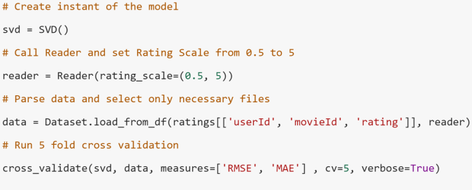
- Step 5- Follow along the below examples
Cheers!


You must be logged in to post a comment.