Linear Discriminant Analysis ( LDA) with Scikit

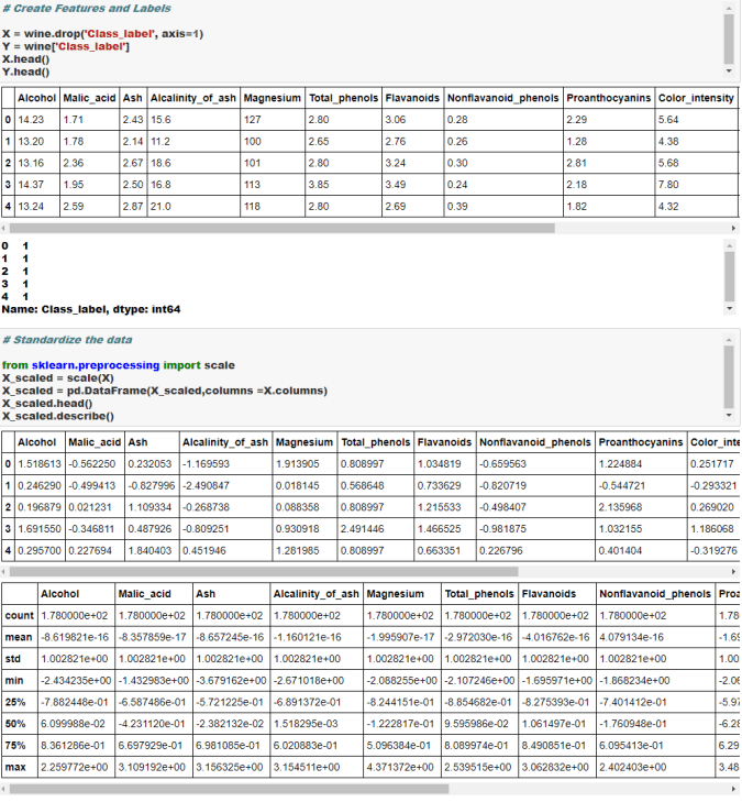
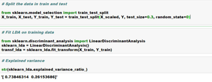
Linear Discriminant Analysis (LDA) is similar to Principal Component Analysis (PCA) in reducing the dimensionality. However, there are certain nuances with LDA that we should be aware of-

  • LDA is supervised (needs categorical dependent variable) to provide the best linear combination of original variables while providing the maximum separation among the different groups. On the other hand, PCA is unsupervised
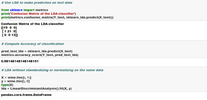
  • LDA can be used for classification also, whereas PCA is generally used for unsupervised learning
  • LDA doesn’t need the numbers of discriminant to be passed on ahead of time. Generally speaking the number of discriminant will be lower of the number of variables or number of categories-1.
  • LDA is more robust and can be conducted without even standardizing or normalizing the variables in certain cases
  • LDA is preferred for bigger data sets and machine learning

Let the action begin now-

lda1LDA2LDA3LDA4LDA5

Cheers!

Logistic Regression using Scikit Python

What Is Logistic Regression?

Logistic regression is a supervised machine learning algorithm used for binary classification — predicting whether an outcome belongs to one of two classes (e.g., survived / did not survive, spam / not spam, fraud / not fraud).

Unlike linear regression, which predicts a continuous value, logistic regression predicts a probability that an observation belongs to the positive class. That probability is then converted into a class label using a decision threshold (typically 0.5).


Use Cases

Logistic regression is widely used when the target is binary or can be treated as binary:

DomainExample
HealthcareDisease diagnosis (positive / negative test result)
FinanceCredit default prediction, fraud detection
MarketingCustomer churn, click-through prediction
HREmployee attrition prediction
TransportationPassenger survival, accident severity classification

In this notebook, we use logistic regression to predict whether a Titanic passenger survived (1) or not (0) based on features such as age, gender, fare, and passenger class.


The Model Equation

Logistic regression starts with a linear combination of features (similar to linear regression):

z = β₀ + β₁x₁ + β₂x₂ + … + βₙxₙ

This value z is passed through the sigmoid (logistic) function to produce a probability between 0 and 1:

P(y = 1 | x) = σ(z) = 1 / (1 + e^(-z))

Where:

  • P(y=1 | x) = probability of the positive class
  • β₀ = intercept (bias term)
  • β₁, β₂, …, βₙ = coefficients (weights) for each feature
  • x₁, x₂, …, xₙ = input feature values

The sigmoid function squashes any real number into the range (0, 1), making it ideal for probability estimation.


Log-Odds (Logit)

Instead of modeling probability directly, logistic regression can be understood as modeling the log-odds (also called the logit) of the outcome:

logit(p) = ln(p / (1 – p)) = β₀ + β₁x₁ + β₂x₂ + … + βₙxₙ

Where:

  • p = probability of the positive class
  • p / (1-p) = odds (ratio of probability of success to probability of failure)
  • ln(p / (1-p)) = log-odds or logit

Key insight: The logit transforms a probability (bounded 0–1) into an unbounded real number, allowing us to use a linear model. A one-unit increase in a feature changes the log-odds by that feature’s coefficient βⱼ.

Example: If β_gender = 1.5, being in the coded “female” category increases the log-odds of survival by 1.5 — which corresponds to multiplying the odds by e^1.5 ≈ 4.48.


Algorithm & Optimization

Logistic regression learns the coefficients β₀, β₁, …, βₙ by maximizing the likelihood of observing the actual training labels — equivalent to minimizing the log-loss (cross-entropy loss):

L = -(1/N) × Σ [ yᵢ log(p̂ᵢ) + (1 – yᵢ) log(1 – p̂ᵢ) ]

Where:

  • N = number of training samples
  • yᵢ = actual label (0 or 1) for sample i
  • p̂ᵢ = predicted probability for sample i

How optimization works:

  1. Initialize coefficients (often to zero or small random values)
  2. Compute predicted probabilities using the sigmoid function
  3. Calculate the loss (log-loss) across all training samples
  4. Compute the gradient (partial derivatives of loss w.r.t. each coefficient)
  5. Update coefficients using an iterative solver such as:
    • L-BFGS (Limited-memory Broyden–Fletcher–Goldfarb–Shanno) — default in scikit-learn
    • Stochastic Gradient Descent (SGD)
    • Newton’s method
  6. Repeat until convergence (loss stops improving)

scikit-learn’s LogisticRegression() uses these solvers under the hood — no manual gradient descent is needed.


Underlying Assumptions

Logistic regression performs best when these assumptions are reasonably met:

AssumptionDescription
Binary outcomeThe dependent variable has only two meaningful classes
Independence of observationsEach row is independent (no repeated measures on the same subject)
Linearity of log-oddsThe log-odds of the outcome is a linear function of the predictors
No perfect multicollinearityPredictors should not be perfectly correlated with each other
Large enough sample sizeRule of thumb: at least 10 events per predictor variable
No extreme outliersOutliers can disproportionately influence coefficient estimates

Violations don’t always make the model unusable, but they can reduce accuracy or make coefficients harder to interpret.


Interpreting Coefficients

Coefficient signMeaning
Positive βⱼIncreases the log-odds (and probability) of the positive class
Negative βⱼDecreases the log-odds (and probability) of the positive class
Magnitudeβⱼ

After training, we examine log.coef_ in this notebook to see which features most strongly predict survival.


Decision Threshold & Probability Output

By default, scikit-learn classifies an observation as class 1 if P(y=1) >= 0.5, otherwise class 0. This threshold can be adjusted:

  • Lower threshold (e.g., 0.3) → more positive predictions (higher recall, lower precision)
  • Higher threshold (e.g., 0.7) → fewer positive predictions (higher precision, lower recall)

predict_proba() returns the raw probabilities, which we use later in this notebook for threshold optimization and detailed prediction analysis.


Logistic Regression vs. Linear Regression

Logistic Regression vs. Linear Regression

AspectLinear RegressionLogistic Regression
OutputContinuous valueProbability (0 to 1)
Link functionIdentitySigmoid (logit)
Loss functionMean Squared ErrorLog-loss (cross-entropy)
Use casePredicting quantitiesBinary classification

Strengths & Limitations

Strengths:

  • Simple, fast, and highly interpretable
  • Outputs well-calibrated probabilities
  • Works well as a baseline classifier
  • Less prone to overfitting with small datasets (with regularization)

Limitations:

  • Assumes a linear decision boundary in log-odds space
  • Struggles with complex non-linear relationships
  • Sensitive to feature scaling (we apply StandardScaler in this notebook)
  • Requires thoughtful handling of missing values and categorical encoding

CODES

# =============================================================================
# IMPORTS AND ENVIRONMENT SETUP
# =============================================================================
# Import core libraries for numerics, data handling, and plotting
import numpy as np
import pandas as pd
from matplotlib import pyplot as plt
import seaborn as sns
#import pandas_profiling
%matplotlib inline
!pip install tqdm

# Enable multiple expressions per cell in Jupyter (shows all results, not just last)
from IPython.core.interactiveshell import InteractiveShell
InteractiveShell.ast_node_interactivity = “all”


# =============================================================================
# EXPLORATORY DATA ANALYSIS — Titanic Dataset Overview
# =============================================================================
# Load a fresh copy of the Titanic dataset for initial exploration
titanic_eda = sns.load_dataset(‘titanic’)

# — Dataset shape and basic statistics —
print(“=” * 60)
print(“TITANIC DATASET — EXPLORATORY DATA ANALYSIS”)
print(“=” * 60)
print(f”\nDataset Shape: {titanic_eda.shape[0]} rows x {titanic_eda.shape[1]} columns”)
print(f”Overall Survival Rate: {titanic_eda[‘survived’].mean():.1%}”)
print(“\n— Missing Values —“)
print(titanic_eda.isna().sum())
print(“\n— Survival by Gender —“)
print(titanic_eda.groupby(‘sex’)[‘survived’].mean().round(3))
print(“\n— Survival by Passenger Class —“)
print(titanic_eda.groupby(‘pclass’)[‘survived’].mean().round(3))

# — Chart 1: Overview panel (survival, gender, class, age) —
fig, axes = plt.subplots(2, 2, figsize=(14, 10))

sns.countplot(data=titanic_eda, x=’survived’, ax=axes[0, 0], palette=’Set2′)
axes[0, 0].set_title(‘Survival Count (0 = Died, 1 = Survived)’)
axes[0, 0].set_xlabel(‘Survived’)

sns.countplot(data=titanic_eda, x=’sex’, hue=’survived’, ax=axes[0, 1], palette=’Set1′)
axes[0, 1].set_title(‘Survival by Gender’)
axes[0, 1].legend(title=’Survived’)

sns.countplot(data=titanic_eda, x=’pclass’, hue=’survived’, ax=axes[1, 0], palette=’Set1′)
axes[1, 0].set_title(‘Survival by Passenger Class’)
axes[1, 0].set_xlabel(‘Passenger Class’)
axes[1, 0].legend(title=’Survived’)

sns.histplot(data=titanic_eda, x=’age’, hue=’survived’, kde=True, ax=axes[1, 1], palette=’Set1′)
axes[1, 1].set_title(‘Age Distribution by Survival Status’)

plt.suptitle(‘Titanic EDA — Key Survival Patterns’, fontsize=14, y=1.02)
plt.tight_layout()
plt.show()

# — Chart 2: Fare distribution and missing values —
fig, axes = plt.subplots(1, 2, figsize=(14, 5))

sns.boxplot(data=titanic_eda, x=’survived’, y=’fare’, ax=axes[0], palette=’Pastel1′)
axes[0].set_title(‘Fare Distribution by Survival Status’)
axes[0].set_xlabel(‘Survived (0 = Died, 1 = Survived)’)

missing = titanic_eda.isna().sum()
missing = missing[missing > 0].sort_values(ascending=False)
missing.plot(kind=’bar’, ax=axes[1], color=’coral’, edgecolor=’black’)
axes[1].set_title(‘Missing Values by Column’)
axes[1].set_ylabel(‘Count’)
axes[1].tick_params(axis=’x’, rotation=45)

plt.tight_layout()
plt.show()

# — Chart 3: Correlation heatmap for numeric features —
numeric_cols = titanic_eda.select_dtypes(include=’number’).columns
corr = titanic_eda[numeric_cols].corr()
plt.figure(figsize=(8, 6))
sns.heatmap(corr, annot=True, fmt=’.2f’, cmap=’coolwarm’, center=0, square=True)
plt.title(‘Correlation Heatmap — Numeric Features’)
plt.tight_layout()
plt.show()


# =============================================================================
# LOAD TITANIC DATA
# =============================================================================
# Load the built-in Titanic dataset from seaborn and preview first/last rows
titanic = sns.load_dataset(‘titanic’)
titanic.head()
titanic.tail()

# =============================================================================
# PROGRESS BAR DEMO (tqdm)
# =============================================================================
# Demonstrate tqdm progress bar utility
from tqdm import tqdm
from time import sleep
with tqdm(total=100) as pbar:
for i in range(10):
sleep(0.1)
pbar.update(10)

# =============================================================================
# DROP REDUNDANT / LEAKAGE COLUMNS
# =============================================================================
# Remove columns that duplicate information or would leak the target variable
# Note: ‘deck’ is kept here because it is imputed later in the missing-value section
titanic.drop([‘alive’, ‘class’,’who’, ’embark_town’, ‘alone’, ‘adult_male’]
,axis=1,inplace=True)


# Preview cleaned dataframe
titanic.head()

# Check data types and non-null counts
titanic.info()

# Explore embarked port distribution before handling missing values
titanic[’embarked’].value_counts()

# Find the most frequent embarkation port (used for imputation)
titanic[’embarked’].mode()

# Inspect rows with missing embarked values
titanic.iloc[[61,684],:]

titanic.info()

# Fill missing embarked values with the mode (most common port: Southampton)
titanic[’embarked’] = titanic[’embarked’].fillna(titanic[’embarked’].mode()[0])

titanic.info()

# Summary of remaining missing values across all columns
titanic.isna().sum()

titanic.shape

# =============================================================================
# REMOVE DUPLICATE ROWS
# =============================================================================
# drop duplicates
titanic = titanic.drop_duplicates()
titanic.shape

# =============================================================================
# EXPLORE MISSING AGE VALUES
# =============================================================================
# Isolate passengers with missing age for inspection
titanic_age_missing = titanic[titanic[‘age’].isna()]
titanic_age_missing.head()
titanic_age_missing.shape

# Inspect specific rows of interest
titanic.iloc[[19,26,28],:]

# =============================================================================
# RENAME COLUMNS FOR CLARITY
# =============================================================================
# Standardize column names to descriptive lowercase labels
titanic = titanic.rename(columns = {“sex”:”gender”, “sibsp”:’siblings_spouse’,
“parch”:”parents_child”,”Survived”:’survived’,
“Pclass”:’plcass’,
‘Age’:’age’,’Fare’:’fare’, ‘Embarked’:’embarked’})
titanic.head()

titanic.info()

titanic.columns

titanic[’embarked’].value_counts()

# =============================================================================
# DECK COLUMN — MISSING VALUE TREATMENT
# =============================================================================
# Convert deck to object type and fill missing deck values with ‘Not Assigned’
# (Must run before categorical encoding so deck is not dropped and median fill works)
titanic.deck = titanic.deck.astype(‘object’)

titanic[‘deck’] = titanic[‘deck’].fillna(‘Not Assigned’)

titanic.info()

titanic.deck.isna().sum()

# =============================================================================
# ENCODE CATEGORICAL VARIABLES AS INTEGER CODES
# =============================================================================
# Convert object-type columns to numeric category codes for modeling
for x in titanic.columns:
if titanic[x].dtype == “object”:
titanic[x]=pd.Categorical(titanic[x]).codes

titanic.head()

# =============================================================================
# IMPUTE MISSING AGE WITH MEDIAN
# =============================================================================
# Compute median age and fill missing age values
titanic[‘age’].median()

titanic[‘age’] = titanic[‘age’].fillna(titanic[‘age’].median())
titanic.info()

# Fill any remaining numeric missing values with column medians
titanic= titanic.fillna(titanic.median())
titanic.info()

titanic.iloc[[19,26,28],:]

# =============================================================================
# HANDLE REMAINING EMBARKED MISSING VALUES
# =============================================================================
titanic_embark_missing = titanic[titanic[’embarked’].isna()]
titanic_embark_missing

titanic[’embarked’].mode()

titanic[’embarked’] = titanic[’embarked’].fillna(titanic[’embarked’].mode()[0])

titanic.iloc[[61,684],:]

# Sample and inspect the cleaned dataset
titanic.head(10)
titanic.sample(10)
titanic.tail(10)
titanic.info()

titanic.columns

titanic.info()

# =============================================================================
# DESCRIPTIVE STATISTICS AND OUTLIER ANALYSIS
# =============================================================================
# Summary statistics for all numeric columns
titanic.describe()

# Percentile distribution to identify potential outliers
titanic.quantile((0, 0.01,0.05, 0.5, 0.95,0.99, 1.0))

# Visualize fare distribution before clipping outliers
titanic.fare.hist()


# Clip fare outliers at the 99th percentile upper bound
titanic.fare = np.clip(titanic.fare,0,249.00622 )

titanic.fare.describe()

titanic.fare.hist()

titanic.info()

titanic.describe()

# Clip all numeric columns to their 1st and 99th percentile bounds
for x in titanic.columns:
outlier = titanic[x].quantile([0.01,0.99]).values
titanic[x] = np.clip(titanic[x], outlier[0], outlier[1])


titanic.describe()

# prompt: read a csv file

#df = pd.read_csv(‘filename.csv’)


titanic.describe()
titanic.head()

# Check class balance of the target variable (survived)
titanic.groupby(‘survived’).size()

titanic.shape

# =============================================================================
# PREPARE FEATURES (X) AND TARGET (y)
# =============================================================================
# Import scikit-learn modules for splitting, metrics, and logistic regression
from sklearn.model_selection import train_test_split
from sklearn import metrics
from sklearn.linear_model import LogisticRegression


# Separate features from target variable
x = titanic.drop([‘survived’], axis = 1, inplace=False)
y = titanic[‘survived’]
x.shape
print(‘\n’)
y.shape

titanic.describe()

# =============================================================================
# FEATURE SCALING — MinMaxScaler (demonstration)
# =============================================================================
from sklearn.preprocessing import MinMaxScaler
scld_titanic = MinMaxScaler(feature_range= (0,1))
titanic_transformed = scld_titanic.fit_transform(x)
scld_titanic_df = pd.DataFrame(titanic_transformed, columns = x.columns)
scld_titanic_df.head()
scld_titanic_df.describe()

# =============================================================================
# FEATURE SCALING — StandardScaler (used for modeling)
# =============================================================================
from sklearn.preprocessing import StandardScaler
scld_titanic = StandardScaler()
titanic_transformed = scld_titanic.fit_transform(x)
scld_titanic_df = pd.DataFrame(titanic_transformed, columns = x.columns)
scld_titanic_df.head()
np.round(scld_titanic_df.describe(),2)

# =============================================================================
# TRAIN / TEST SPLIT
# =============================================================================
# Split in Train and Test data
x_train, x_test, y_train, y_test = train_test_split(scld_titanic_df, y, test_size=0.2, random_state=999)
x_train.shape
y_train.shape
x_test.shape
y_test.shape

x_train
y_train
x_test

# Check survival rate (% positive class) in train and test sets
np.round(y_train.sum()/y_train.count()*100,2)
print(‘\n’)
np.round(y_test.sum()/y_test.count()*100,2)

# =============================================================================
# LOGISTIC REGRESSION MODEL
# =============================================================================
# Initialize logistic regression classifier
log = LogisticRegression()

log

# Fit the model on training data
log.fit(x_train, y_train)

# =============================================================================
# PREDICTIONS AND EVALUATION
# =============================================================================
# Generate class predictions on the test set
predicted = log.predict(x_test)
predicted

from sklearn import metrics
print((metrics.classification_report(y_test, predicted)))

# Build confusion matrix comparing actual vs predicted labels
df_confusion = metrics.confusion_matrix(y_test,predicted)
df_confusion


import seaborn as sns
import matplotlib.pyplot as plt
# Visualize confusion matrix as a heatmap
sns.heatmap(df_confusion, cmap = ‘Greens’,xticklabels=[‘Prediction No’,’Prediction Yes’],
yticklabels=[‘Actual No’,’Actual Yes’], annot=True, fmt=’d’)
plt.show();

# Overall accuracy score
metrics.accuracy_score(y_test, predicted)

# =============================================================================
# MODEL INTERPRETATION — COEFFICIENTS
# =============================================================================
# Raw model coefficients (log-odds impact of each feature)
log.coef_

x.columns

# Combine feature names with their coefficients for readability
coeff = pd.concat([pd.DataFrame(x.columns), pd.DataFrame(np.transpose(log.coef_))],axis =1 )
coeff.columns = (“Variable”, ‘Coeff’)

coeff

# =============================================================================
# PROBABILITY PREDICTIONS AND THRESHOLD ANALYSIS
# =============================================================================
# Find out probability of the classes and predicted classes
predicted_prob = log.predict_proba(x_test)
predicted_prob_df = pd.DataFrame(predicted_prob)
predicted_classes_df = pd.DataFrame(predicted)
y_actual_df = pd.DataFrame(y_test.values)
predicted_df = pd.concat([predicted_prob_df, predicted_classes_df, y_actual_df], axis=1)
predicted_df.columns = [‘Prob_0′,’Prob_1′,’Predicted_Class’, ‘Actual_Class’]
predicted_df.sample(20)


predicted_prob

Output Block

Requirement already satisfied: tqdm in /usr/local/lib/python3.12/dist-packages (4.67.3)
============================================================
TITANIC DATASET — EXPLORATORY DATA ANALYSIS
============================================================

Dataset Shape: 891 rows x 15 columns
Overall Survival Rate: 38.4%

— Missing Values —
survived 0
pclass 0
sex 0
age 177
sibsp 0
parch 0
fare 0
embarked 2
class 0
who 0
adult_male 0
deck 688
embark_town 2
alive 0
alone 0
dtype: int64

— Survival by Gender —
sex
female 0.742
male 0.189
Name: survived, dtype: float64

— Survival by Passenger Class —
pclass
1 0.630
2 0.473
3 0.242
Name: survived, dtype: float64
/tmp/ipykernel_597/1527970602.py:40: FutureWarning:

Passing `palette` without assigning `hue` is deprecated and will be removed in v0.14.0. Assign the `x` variable to `hue` and set `legend=False` for the same effect.

sns.countplot(data=titanic_eda, x=’survived’, ax=axes[0, 0], palette=’Set2′)

/tmp/ipykernel_597/1527970602.py:63: FutureWarning:

Passing `palette` without assigning `hue` is deprecated and will be removed in v0.14.0. Assign the `x` variable to `hue` and set `legend=False` for the same effect.

sns.boxplot(data=titanic_eda, x=’survived’, y=’fare’, ax=axes[0], palette=’Pastel1′)


100%|██████████| 100/100 [00:01<00:00, 98.40it/s]
<class ‘pandas.core.frame.DataFrame’>
RangeIndex: 891 entries, 0 to 890
Data columns (total 9 columns):
# Column Non-Null Count Dtype
— —— ————– —–
0 survived 891 non-null int64
1 pclass 891 non-null int64
2 sex 891 non-null object
3 age 714 non-null float64
4 sibsp 891 non-null int64
5 parch 891 non-null int64
6 fare 891 non-null float64
7 embarked 889 non-null object
8 deck 203 non-null category
dtypes: category(1), float64(2), int64(4), object(2)
memory usage: 57.0+ KB
<class ‘pandas.core.frame.DataFrame’>
RangeIndex: 891 entries, 0 to 890
Data columns (total 9 columns):
# Column Non-Null Count Dtype
— —— ————– —–
0 survived 891 non-null int64
1 pclass 891 non-null int64
2 sex 891 non-null object
3 age 714 non-null float64
4 sibsp 891 non-null int64
5 parch 891 non-null int64
6 fare 891 non-null float64
7 embarked 889 non-null object
8 deck 203 non-null category
dtypes: category(1), float64(2), int64(4), object(2)
memory usage: 57.0+ KB
<class ‘pandas.core.frame.DataFrame’>
RangeIndex: 891 entries, 0 to 890
Data columns (total 9 columns):
# Column Non-Null Count Dtype
— —— ————– —–
0 survived 891 non-null int64
1 pclass 891 non-null int64
2 sex 891 non-null object
3 age 714 non-null float64
4 sibsp 891 non-null int64
5 parch 891 non-null int64
6 fare 891 non-null float64
7 embarked 891 non-null object
8 deck 203 non-null category
dtypes: category(1), float64(2), int64(4), object(2)
memory usage: 57.0+ KB
<class ‘pandas.core.frame.DataFrame’>
Index: 784 entries, 0 to 890
Data columns (total 9 columns):
# Column Non-Null Count Dtype
— —— ————– —–
0 survived 784 non-null int64
1 pclass 784 non-null int64
2 gender 784 non-null object
3 age 678 non-null float64
4 siblings_spouse 784 non-null int64
5 parents_child 784 non-null int64
6 fare 784 non-null float64
7 embarked 784 non-null object
8 deck 202 non-null category
dtypes: category(1), float64(2), int64(4), object(2)
memory usage: 56.2+ KB
<class ‘pandas.core.frame.DataFrame’>
Index: 784 entries, 0 to 890
Data columns (total 9 columns):
# Column Non-Null Count Dtype
— —— ————– —–
0 survived 784 non-null int64
1 pclass 784 non-null int64
2 gender 784 non-null object
3 age 678 non-null float64
4 siblings_spouse 784 non-null int64
5 parents_child 784 non-null int64
6 fare 784 non-null float64
7 embarked 784 non-null object
8 deck 784 non-null object
dtypes: float64(2), int64(4), object(3)
memory usage: 61.2+ KB
<class ‘pandas.core.frame.DataFrame’>
Index: 784 entries, 0 to 890
Data columns (total 9 columns):
# Column Non-Null Count Dtype
— —— ————– —–
0 survived 784 non-null int64
1 pclass 784 non-null int64
2 gender 784 non-null int8
3 age 784 non-null float64
4 siblings_spouse 784 non-null int64
5 parents_child 784 non-null int64
6 fare 784 non-null float64
7 embarked 784 non-null int8
8 deck 784 non-null int8
dtypes: float64(2), int64(4), int8(3)
memory usage: 45.2 KB
<class ‘pandas.core.frame.DataFrame’>
Index: 784 entries, 0 to 890
Data columns (total 9 columns):
# Column Non-Null Count Dtype
— —— ————– —–
0 survived 784 non-null int64
1 pclass 784 non-null int64
2 gender 784 non-null int8
3 age 784 non-null float64
4 siblings_spouse 784 non-null int64
5 parents_child 784 non-null int64
6 fare 784 non-null float64
7 embarked 784 non-null int8
8 deck 784 non-null int8
dtypes: float64(2), int64(4), int8(3)
memory usage: 45.2 KB
<class ‘pandas.core.frame.DataFrame’>
Index: 784 entries, 0 to 890
Data columns (total 9 columns):
# Column Non-Null Count Dtype
— —— ————– —–
0 survived 784 non-null int64
1 pclass 784 non-null int64
2 gender 784 non-null int8
3 age 784 non-null float64
4 siblings_spouse 784 non-null int64
5 parents_child 784 non-null int64
6 fare 784 non-null float64
7 embarked 784 non-null int8
8 deck 784 non-null int8
dtypes: float64(2), int64(4), int8(3)
memory usage: 45.2 KB
<class ‘pandas.core.frame.DataFrame’>
Index: 784 entries, 0 to 890
Data columns (total 9 columns):
# Column Non-Null Count Dtype
— —— ————– —–
0 survived 784 non-null int64
1 pclass 784 non-null int64
2 gender 784 non-null int8
3 age 784 non-null float64
4 siblings_spouse 784 non-null int64
5 parents_child 784 non-null int64
6 fare 784 non-null float64
7 embarked 784 non-null int8
8 deck 784 non-null int8
dtypes: float64(2), int64(4), int8(3)
memory usage: 45.2 KB
<class ‘pandas.core.frame.DataFrame’>
Index: 784 entries, 0 to 890
Data columns (total 9 columns):
# Column Non-Null Count Dtype
— —— ————– —–
0 survived 784 non-null int64
1 pclass 784 non-null int64
2 gender 784 non-null int8
3 age 784 non-null float64
4 siblings_spouse 784 non-null int64
5 parents_child 784 non-null int64
6 fare 784 non-null float64
7 embarked 784 non-null int8
8 deck 784 non-null int8
dtypes: float64(2), int64(4), int8(3)
memory usage: 45.2 KB


precision recall f1-score support

0 0.79 0.83 0.81 90
1 0.76 0.70 0.73 67

accuracy 0.78 157
macro avg 0.77 0.77 0.77 157
weighted avg 0.78 0.78 0.78 157


array([[0.55397344, 0.44602656],
[0.36648402, 0.63351598],
[0.82161992, 0.17838008],
[0.14546149, 0.85453851],
[0.84317581, 0.15682419],
[0.85898305, 0.14101695],
[0.1203916 , 0.8796084 ],
[0.53805585, 0.46194415],
[0.35717302, 0.64282698],
[0.32849211, 0.67150789],
[0.8049969 , 0.1950031 ],
[0.91066252, 0.08933748],
[0.14053402, 0.85946598],
[0.80303192, 0.19696808],
[0.20489829, 0.79510171],
[0.53863242, 0.46136758],
[0.83888713, 0.16111287],
[0.74881101, 0.25118899],
[0.87802515, 0.12197485],
[0.06159685, 0.93840315],
[0.27139185, 0.72860815],
[0.86190473, 0.13809527],
[0.75697559, 0.24302441],
[0.54108302, 0.45891698],
[0.44893086, 0.55106914],
[0.24285506, 0.75714494],
[0.92521486, 0.07478514],
[0.44515852, 0.55484148],
[0.91673444, 0.08326556],
[0.88859559, 0.11140441],
[0.94591075, 0.05408925],
[0.93521218, 0.06478782],
[0.62625257, 0.37374743],
[0.92211925, 0.07788075],
[0.45685666, 0.54314334],
[0.84312216, 0.15687784],
[0.88547452, 0.11452548],
[0.30936126, 0.69063874],
[0.07939955, 0.92060045],
[0.93219874, 0.06780126],
[0.63330031, 0.36669969],
[0.92053872, 0.07946128],
[0.92868217, 0.07131783],
[0.5183927 , 0.4816073 ],
[0.1146845 , 0.8853155 ],
[0.72566823, 0.27433177],
[0.48886081, 0.51113919],
[0.16107575, 0.83892425],
[0.53904267, 0.46095733],
[0.72140052, 0.27859948],
[0.62960379, 0.37039621],
[0.89962517, 0.10037483],
[0.38187136, 0.61812864],
[0.84040645, 0.15959355],
[0.83113253, 0.16886747],
[0.37034959, 0.62965041],
[0.70190266, 0.29809734],
[0.77624547, 0.22375453],
[0.43187485, 0.56812515],
[0.07140916, 0.92859084],
[0.20527775, 0.79472225],
[0.61233815, 0.38766185],
[0.88753928, 0.11246072],
[0.37644464, 0.62355536],
[0.94206494, 0.05793506],
[0.24231454, 0.75768546],
[0.38422862, 0.61577138],
[0.89253394, 0.10746606],
[0.91772881, 0.08227119],
[0.81285549, 0.18714451],
[0.42634743, 0.57365257],
[0.52135864, 0.47864136],
[0.84618193, 0.15381807],
[0.67191945, 0.32808055],
[0.24777467, 0.75222533],
[0.34002452, 0.65997548],
[0.84284584, 0.15715416],
[0.80420694, 0.19579306],
[0.32039026, 0.67960974],
[0.33664048, 0.66335952],
[0.89465304, 0.10534696],
[0.85935537, 0.14064463],
[0.58474389, 0.41525611],
[0.38899587, 0.61100413],
[0.26705897, 0.73294103],
[0.13009479, 0.86990521],
[0.20701663, 0.79298337],
[0.18618385, 0.81381615],
[0.74663678, 0.25336322],
[0.74368753, 0.25631247],
[0.58907781, 0.41092219],
[0.12987609, 0.87012391],
[0.8431743 , 0.1568257 ],
[0.18348496, 0.81651504],
[0.03473669, 0.96526331],
[0.59965075, 0.40034925],
[0.90786111, 0.09213889],
[0.40560793, 0.59439207],
[0.9645318 , 0.0354682 ],
[0.95093358, 0.04906642],
[0.23132857, 0.76867143],
[0.92231606, 0.07768394],
[0.74551094, 0.25448906],
[0.879819 , 0.120181 ],
[0.65771473, 0.34228527],
[0.10796858, 0.89203142],
[0.89633336, 0.10366664],
[0.19389314, 0.80610686],
[0.94162223, 0.05837777],
[0.58125657, 0.41874343],
[0.17418465, 0.82581535],
[0.89577491, 0.10422509],
[0.84518367, 0.15481633],
[0.80321262, 0.19678738],
[0.76732066, 0.23267934],
[0.83516388, 0.16483612],
[0.75066159, 0.24933841],
[0.2825069 , 0.7174931 ],
[0.42468534, 0.57531466],
[0.85903103, 0.14096897],
[0.5367603 , 0.4632397 ],
[0.89319696, 0.10680304],
[0.41541597, 0.58458403],
[0.91095574, 0.08904426],
[0.85926671, 0.14073329],
[0.15205884, 0.84794116],
[0.837398 , 0.162602 ],
[0.82548683, 0.17451317],
[0.10576671, 0.89423329],
[0.91733691, 0.08266309],
[0.05606322, 0.94393678],
[0.85412342, 0.14587658],
[0.93426411, 0.06573589],
[0.46850755, 0.53149245],
[0.16914952, 0.83085048],
[0.12045064, 0.87954936],
[0.88320405, 0.11679595],
[0.20782634, 0.79217366],
[0.4068325 , 0.5931675 ],
[0.41507059, 0.58492941],
[0.61600861, 0.38399139],
[0.35813055, 0.64186945],
[0.53540125, 0.46459875],
[0.60871701, 0.39128299],
[0.84317102, 0.15682898],
[0.24748414, 0.75251586],
[0.78007734, 0.21992266],
[0.91667162, 0.08332838],
[0.15029365, 0.84970635],
[0.04810056, 0.95189944],
[0.89427977, 0.10572023],
[0.56399894, 0.43600106],
[0.90422189, 0.09577811],
[0.9671217 , 0.0328783 ],
[0.93949532, 0.06050468],
[0.0861572 , 0.9138428 ],
[0.46135897, 0.53864103]])

Requirement already satisfied: tqdm in /usr/local/lib/python3.12/dist-packages (4.67.3)
============================================================
TITANIC DATASET — EXPLORATORY DATA ANALYSIS
============================================================

Dataset Shape: 891 rows x 15 columns
Overall Survival Rate: 38.4%

--- Missing Values ---
survived         0
pclass           0
sex              0
age            177
sibsp            0
parch            0
fare             0
embarked         2
class            0
who              0
adult_male       0
deck           688
embark_town      2
alive            0
alone            0
dtype: int64

--- Survival by Gender ---
sex
female    0.742
male      0.189
Name: survived, dtype: float64

--- Survival by Passenger Class ---
pclass
1    0.630
2    0.473
3    0.242
Name: survived, dtype: float64
/tmp/ipykernel_597/1527970602.py:40: FutureWarning: 

Passing `palette` without assigning `hue` is deprecated and will be removed in v0.14.0. Assign the `x` variable to `hue` and set `legend=False` for the same effect.

  sns.countplot(data=titanic_eda, x='survived', ax=axes[0, 0], palette='Set2')
/tmp/ipykernel_597/1527970602.py:63: FutureWarning: 

Passing `palette` without assigning `hue` is deprecated and will be removed in v0.14.0. Assign the `x` variable to `hue` and set `legend=False` for the same effect.

  sns.boxplot(data=titanic_eda, x='survived', y='fare', ax=axes[0], palette='Pastel1')
100%|██████████| 100/100 [00:01<00:00, 98.40it/s]
<class 'pandas.core.frame.DataFrame'>
RangeIndex: 891 entries, 0 to 890
Data columns (total 9 columns):
 #   Column    Non-Null Count  Dtype   
---  ------    --------------  -----   
 0   survived  891 non-null    int64   
 1   pclass    891 non-null    int64   
 2   sex       891 non-null    object  
 3   age       714 non-null    float64 
 4   sibsp     891 non-null    int64   
 5   parch     891 non-null    int64   
 6   fare      891 non-null    float64 
 7   embarked  889 non-null    object  
 8   deck      203 non-null    category
dtypes: category(1), float64(2), int64(4), object(2)
memory usage: 57.0+ KB
<class 'pandas.core.frame.DataFrame'>
RangeIndex: 891 entries, 0 to 890
Data columns (total 9 columns):
 #   Column    Non-Null Count  Dtype   
---  ------    --------------  -----   
 0   survived  891 non-null    int64   
 1   pclass    891 non-null    int64   
 2   sex       891 non-null    object  
 3   age       714 non-null    float64 
 4   sibsp     891 non-null    int64   
 5   parch     891 non-null    int64   
 6   fare      891 non-null    float64 
 7   embarked  889 non-null    object  
 8   deck      203 non-null    category
dtypes: category(1), float64(2), int64(4), object(2)
memory usage: 57.0+ KB
<class 'pandas.core.frame.DataFrame'>
RangeIndex: 891 entries, 0 to 890
Data columns (total 9 columns):
 #   Column    Non-Null Count  Dtype   
---  ------    --------------  -----   
 0   survived  891 non-null    int64   
 1   pclass    891 non-null    int64   
 2   sex       891 non-null    object  
 3   age       714 non-null    float64 
 4   sibsp     891 non-null    int64   
 5   parch     891 non-null    int64   
 6   fare      891 non-null    float64 
 7   embarked  891 non-null    object  
 8   deck      203 non-null    category
dtypes: category(1), float64(2), int64(4), object(2)
memory usage: 57.0+ KB
<class 'pandas.core.frame.DataFrame'>
Index: 784 entries, 0 to 890
Data columns (total 9 columns):
 #   Column           Non-Null Count  Dtype   
---  ------           --------------  -----   
 0   survived         784 non-null    int64   
 1   pclass           784 non-null    int64   
 2   gender           784 non-null    object  
 3   age              678 non-null    float64 
 4   siblings_spouse  784 non-null    int64   
 5   parents_child    784 non-null    int64   
 6   fare             784 non-null    float64 
 7   embarked         784 non-null    object  
 8   deck             202 non-null    category
dtypes: category(1), float64(2), int64(4), object(2)
memory usage: 56.2+ KB
<class 'pandas.core.frame.DataFrame'>
Index: 784 entries, 0 to 890
Data columns (total 9 columns):
 #   Column           Non-Null Count  Dtype  
---  ------           --------------  -----  
 0   survived         784 non-null    int64  
 1   pclass           784 non-null    int64  
 2   gender           784 non-null    object 
 3   age              678 non-null    float64
 4   siblings_spouse  784 non-null    int64  
 5   parents_child    784 non-null    int64  
 6   fare             784 non-null    float64
 7   embarked         784 non-null    object 
 8   deck             784 non-null    object 
dtypes: float64(2), int64(4), object(3)
memory usage: 61.2+ KB
<class 'pandas.core.frame.DataFrame'>
Index: 784 entries, 0 to 890
Data columns (total 9 columns):
 #   Column           Non-Null Count  Dtype  
---  ------           --------------  -----  
 0   survived         784 non-null    int64  
 1   pclass           784 non-null    int64  
 2   gender           784 non-null    int8   
 3   age              784 non-null    float64
 4   siblings_spouse  784 non-null    int64  
 5   parents_child    784 non-null    int64  
 6   fare             784 non-null    float64
 7   embarked         784 non-null    int8   
 8   deck             784 non-null    int8   
dtypes: float64(2), int64(4), int8(3)
memory usage: 45.2 KB
<class 'pandas.core.frame.DataFrame'>
Index: 784 entries, 0 to 890
Data columns (total 9 columns):
 #   Column           Non-Null Count  Dtype  
---  ------           --------------  -----  
 0   survived         784 non-null    int64  
 1   pclass           784 non-null    int64  
 2   gender           784 non-null    int8   
 3   age              784 non-null    float64
 4   siblings_spouse  784 non-null    int64  
 5   parents_child    784 non-null    int64  
 6   fare             784 non-null    float64
 7   embarked         784 non-null    int8   
 8   deck             784 non-null    int8   
dtypes: float64(2), int64(4), int8(3)
memory usage: 45.2 KB
<class 'pandas.core.frame.DataFrame'>
Index: 784 entries, 0 to 890
Data columns (total 9 columns):
 #   Column           Non-Null Count  Dtype  
---  ------           --------------  -----  
 0   survived         784 non-null    int64  
 1   pclass           784 non-null    int64  
 2   gender           784 non-null    int8   
 3   age              784 non-null    float64
 4   siblings_spouse  784 non-null    int64  
 5   parents_child    784 non-null    int64  
 6   fare             784 non-null    float64
 7   embarked         784 non-null    int8   
 8   deck             784 non-null    int8   
dtypes: float64(2), int64(4), int8(3)
memory usage: 45.2 KB
<class 'pandas.core.frame.DataFrame'>
Index: 784 entries, 0 to 890
Data columns (total 9 columns):
 #   Column           Non-Null Count  Dtype  
---  ------           --------------  -----  
 0   survived         784 non-null    int64  
 1   pclass           784 non-null    int64  
 2   gender           784 non-null    int8   
 3   age              784 non-null    float64
 4   siblings_spouse  784 non-null    int64  
 5   parents_child    784 non-null    int64  
 6   fare             784 non-null    float64
 7   embarked         784 non-null    int8   
 8   deck             784 non-null    int8   
dtypes: float64(2), int64(4), int8(3)
memory usage: 45.2 KB
<class 'pandas.core.frame.DataFrame'>
Index: 784 entries, 0 to 890
Data columns (total 9 columns):
 #   Column           Non-Null Count  Dtype  
---  ------           --------------  -----  
 0   survived         784 non-null    int64  
 1   pclass           784 non-null    int64  
 2   gender           784 non-null    int8   
 3   age              784 non-null    float64
 4   siblings_spouse  784 non-null    int64  
 5   parents_child    784 non-null    int64  
 6   fare             784 non-null    float64
 7   embarked         784 non-null    int8   
 8   deck             784 non-null    int8   
dtypes: float64(2), int64(4), int8(3)
memory usage: 45.2 KB


              precision    recall  f1-score   support

           0       0.79      0.83      0.81        90
           1       0.76      0.70      0.73        67

    accuracy                           0.78       157
   macro avg       0.77      0.77      0.77       157
weighted avg       0.78      0.78      0.78       157

array([[0.55397344, 0.44602656],
[0.36648402, 0.63351598],
[0.82161992, 0.17838008],
[0.14546149, 0.85453851],
[0.84317581, 0.15682419],
[0.85898305, 0.14101695],
[0.1203916 , 0.8796084 ],
[0.53805585, 0.46194415],
[0.35717302, 0.64282698],
[0.32849211, 0.67150789],
[0.8049969 , 0.1950031 ],
[0.91066252, 0.08933748],
[0.14053402, 0.85946598],
[0.80303192, 0.19696808],
[0.20489829, 0.79510171],
[0.53863242, 0.46136758],
[0.83888713, 0.16111287],
[0.74881101, 0.25118899],
[0.87802515, 0.12197485],
[0.06159685, 0.93840315],
[0.27139185, 0.72860815],
[0.86190473, 0.13809527],
[0.75697559, 0.24302441],
[0.54108302, 0.45891698],
[0.44893086, 0.55106914],
[0.24285506, 0.75714494],
[0.92521486, 0.07478514],
[0.44515852, 0.55484148],
[0.91673444, 0.08326556],
[0.88859559, 0.11140441],
[0.94591075, 0.05408925],
[0.93521218, 0.06478782],
[0.62625257, 0.37374743],
[0.92211925, 0.07788075],
[0.45685666, 0.54314334],
[0.84312216, 0.15687784],
[0.88547452, 0.11452548],
[0.30936126, 0.69063874],
[0.07939955, 0.92060045],
[0.93219874, 0.06780126],
[0.63330031, 0.36669969],
[0.92053872, 0.07946128],
[0.92868217, 0.07131783],
[0.5183927 , 0.4816073 ],
[0.1146845 , 0.8853155 ],
[0.72566823, 0.27433177],
[0.48886081, 0.51113919],
[0.16107575, 0.83892425],
[0.53904267, 0.46095733],
[0.72140052, 0.27859948],
[0.62960379, 0.37039621],
[0.89962517, 0.10037483],
[0.38187136, 0.61812864],
[0.84040645, 0.15959355],
[0.83113253, 0.16886747],
[0.37034959, 0.62965041],
[0.70190266, 0.29809734],
[0.77624547, 0.22375453],
[0.43187485, 0.56812515],
[0.07140916, 0.92859084],
[0.20527775, 0.79472225],
[0.61233815, 0.38766185],
[0.88753928, 0.11246072],
[0.37644464, 0.62355536],
[0.94206494, 0.05793506],
[0.24231454, 0.75768546],
[0.38422862, 0.61577138],
[0.89253394, 0.10746606],
[0.91772881, 0.08227119],
[0.81285549, 0.18714451],
[0.42634743, 0.57365257],
[0.52135864, 0.47864136],
[0.84618193, 0.15381807],
[0.67191945, 0.32808055],
[0.24777467, 0.75222533],
[0.34002452, 0.65997548],
[0.84284584, 0.15715416],
[0.80420694, 0.19579306],
[0.32039026, 0.67960974],
[0.33664048, 0.66335952],
[0.89465304, 0.10534696],
[0.85935537, 0.14064463],
[0.58474389, 0.41525611],
[0.38899587, 0.61100413],
[0.26705897, 0.73294103],
[0.13009479, 0.86990521],
[0.20701663, 0.79298337],
[0.18618385, 0.81381615],
[0.74663678, 0.25336322],
[0.74368753, 0.25631247],
[0.58907781, 0.41092219],
[0.12987609, 0.87012391],
[0.8431743 , 0.1568257 ],
[0.18348496, 0.81651504],
[0.03473669, 0.96526331],
[0.59965075, 0.40034925],
[0.90786111, 0.09213889],
[0.40560793, 0.59439207],
[0.9645318 , 0.0354682 ],
[0.95093358, 0.04906642],
[0.23132857, 0.76867143],
[0.92231606, 0.07768394],
[0.74551094, 0.25448906],
[0.879819 , 0.120181 ],
[0.65771473, 0.34228527],
[0.10796858, 0.89203142],
[0.89633336, 0.10366664],
[0.19389314, 0.80610686],
[0.94162223, 0.05837777],
[0.58125657, 0.41874343],
[0.17418465, 0.82581535],
[0.89577491, 0.10422509],
[0.84518367, 0.15481633],
[0.80321262, 0.19678738],
[0.76732066, 0.23267934],
[0.83516388, 0.16483612],
[0.75066159, 0.24933841],
[0.2825069 , 0.7174931 ],
[0.42468534, 0.57531466],
[0.85903103, 0.14096897],
[0.5367603 , 0.4632397 ],
[0.89319696, 0.10680304],
[0.41541597, 0.58458403],
[0.91095574, 0.08904426],
[0.85926671, 0.14073329],
[0.15205884, 0.84794116],
[0.837398 , 0.162602 ],
[0.82548683, 0.17451317],
[0.10576671, 0.89423329],
[0.91733691, 0.08266309],
[0.05606322, 0.94393678],
[0.85412342, 0.14587658],
[0.93426411, 0.06573589],
[0.46850755, 0.53149245],
[0.16914952, 0.83085048],
[0.12045064, 0.87954936],
[0.88320405, 0.11679595],
[0.20782634, 0.79217366],
[0.4068325 , 0.5931675 ],
[0.41507059, 0.58492941],
[0.61600861, 0.38399139],
[0.35813055, 0.64186945],
[0.53540125, 0.46459875],
[0.60871701, 0.39128299],
[0.84317102, 0.15682898],
[0.24748414, 0.75251586],
[0.78007734, 0.21992266],
[0.91667162, 0.08332838],
[0.15029365, 0.84970635],
[0.04810056, 0.95189944],
[0.89427977, 0.10572023],
[0.56399894, 0.43600106],
[0.90422189, 0.09577811],
[0.9671217 , 0.0328783 ],
[0.93949532, 0.06050468],
[0.0861572 , 0.9138428 ],
[0.46135897, 0.53864103]])

Intercepts for the Logistic Regression

plt.figure(figsize=(10, 6))
sns.barplot(x='Variable', y='Coeff', data=coeff, palette='viridis')
plt.title('Logistic Regression Coefficients (with Intercept)')
plt.xlabel('Feature Variables')
plt.ylabel('Coefficient Value')
plt.xticks(rotation=45, ha='right')
plt.tight_layout()
plt.show()
<Figure size 1000x600 with 0 Axes>
/tmp/ipykernel_597/2760321974.py:2: FutureWarning: 

Passing `palette` without assigning `hue` is deprecated and will be removed in v0.14.0. Assign the `x` variable to `hue` and set `legend=False` for the same effect.

  sns.barplot(x='Variable', y='Coeff', data=coeff, palette='viridis')
<Axes: xlabel='Variable', ylabel='Coeff'>
Text(0.5, 1.0, 'Logistic Regression Coefficients (with Intercept)')
Text(0.5, 0, 'Feature Variables')
Text(0, 0.5, 'Coefficient Value')
([0, 1, 2, 3, 4, 5, 6, 7, 8],
 [Text(0, 0, 'pclass'),
  Text(1, 0, 'gender'),
  Text(2, 0, 'age'),
  Text(3, 0, 'siblings_spouse'),
  Text(4, 0, 'parents_child'),
  Text(5, 0, 'fare'),
  Text(6, 0, 'embarked'),
  Text(7, 0, 'deck'),
  Text(8, 0, 'Intercept')])