Data standardization or normalization plays a critical role in most of the statistical analysis and modeling. Let’s spend sometime to talk about the difference between the standardization and normalization first.

Standardization is when a variable is made to follow the standard normal distribution ( mean =0  and standard deviation = 1). On the other hand, normalization is when a variable is fitted within a certain range ( generally between 0 and 1). Here are more details of the above.

Let’s now talk about why we need to do the standardization or normalization before many statistical analysis?

1. In a multivariate analysis when variables have widely different scales, variable(s) with higher range may overshadow the other variables in analysis. For example, let’s say variable X has a range of 0-1000 and variable Y has a range of 0-10. In all likelihood, variable X will outweigh variable Y due to it’s higher range. However, if we standardize or normalize the variable, then we can overcome this issue.
2. Any algorithms which are based on distance computations such as clustering, k nearest neigbour ( KNN), principal component ( PCA) will be greatly affected if you don’t normalize the data
3. Neural networks and deep learning networks also need the variables to be normalized for converging faster and giving more accurate results
4. Multivariate models may become more stable and the coefficients more reliable if you normalize the data
5. It provides immunity from the problem of outliers

Let’s look at a Python example on how we can normalize data-

# MinMaxScaler on California Housing — before vs after
# Formula: x_scaled = (x - min) / (max - min)  ->  values land in [0, 1]
# In Jupyter: add `%matplotlib inline` at the top for inline charts.
import warnings
import matplotlib.pyplot as plt
import pandas as pd
import seaborn as sns
from sklearn.datasets import fetch_california_housing
from sklearn.preprocessing import MinMaxScaler
warnings.filterwarnings("ignore")
sns.set_theme(style="whitegrid")
# 1. Load features
housing = fetch_california_housing()
X = pd.DataFrame(housing.data, columns=housing.feature_names)
print("BEFORE MinMaxScaler (original values):\n")
print(X.head().round(3))
print("\n", X.describe().round(3))
# 2. Fit MinMaxScaler and transform
scaler = MinMaxScaler()
X_scaled = pd.DataFrame(
    scaler.fit_transform(X),
    columns=X.columns,
)
print("\n" + "=" * 50)
print("AFTER MinMaxScaler (scaled to [0, 1]):\n")
print(X_scaled.head().round(3))
print("\n", X_scaled.describe().round(3))
# 3. Worked example — one feature, first 5 rows
feature = "MedInc"
lo = scaler.data_min_[X.columns.get_loc(feature)]
hi = scaler.data_max_[X.columns.get_loc(feature)]
example = pd.DataFrame({
    "raw": X[feature].head(),
    "min": lo,
    "max": hi,
})
example["scaled = (raw - min) / (max - min)"] = (
    (example["raw"] - example["min"]) / (example["max"] - example["min"])
).round(3)
example["sklearn output"] = X_scaled[feature].head().round(3).values
print("\n" + "=" * 50)
print(f"How scaling works for {feature}:\n")
print(example.to_string())
# 4. Quick before / after summary
print("\n" + "=" * 50)
print("Before vs after (min and max per feature):\n")
comparison = pd.DataFrame({
    "before_min": X.min(),
    "before_max": X.max(),
    "after_min": X_scaled.min(),
    "after_max": X_scaled.max(),
}).round(3)
print(comparison.to_string())
# 5. Plots
fig, axes = plt.subplots(1, 2, figsize=(12, 5))
sns.boxplot(data=X, ax=axes[0], color="steelblue", fliersize=2)
axes[0].set_title("Before scaling")
axes[0].set_xticklabels(axes[0].get_xticklabels(), rotation=45, ha="right")
sns.boxplot(data=X_scaled, ax=axes[1], color="darkorange", fliersize=2)
axes[1].set_title("After MinMaxScaler [0, 1]")
axes[1].set_xticklabels(axes[1].get_xticklabels(), rotation=45, ha="right")
plt.suptitle("California Housing — all features", y=1.02)
plt.tight_layout()
plt.show()
fig, axes = plt.subplots(1, 2, figsize=(10, 4))
sns.histplot(X[feature], bins=40, kde=True, ax=axes[0], color="steelblue")
axes[0].set_title(f"Before — {feature}")
axes[0].set_xlabel(feature)
sns.histplot(X_scaled[feature], bins=40, kde=True, ax=axes[1], color="darkorange")
axes[1].set_title(f"After — {feature}")
axes[1].set_xlabel(f"{feature} (scaled)")
plt.tight_layout()
plt.show()
print("\nTakeaway: every feature is rescaled to the same [0, 1] range.")
print("  x_scaled = (x - column_min) / (column_max - column_min)")

BEFORE MinMaxScaler (original values):

   MedInc  HouseAge  AveRooms  AveBedrms  Population  AveOccup  Latitude  \
0   8.325      41.0     6.984      1.024       322.0     2.556     37.88   
1   8.301      21.0     6.238      0.972      2401.0     2.110     37.86   
2   7.257      52.0     8.288      1.073       496.0     2.802     37.85   
3   5.643      52.0     5.817      1.073       558.0     2.548     37.85   
4   3.846      52.0     6.282      1.081       565.0     2.181     37.85   

   Longitude  
0    -122.23  
1    -122.22  
2    -122.24  
3    -122.25  
4    -122.25  

           MedInc   HouseAge   AveRooms  AveBedrms  Population   AveOccup  \
count  20640.000  20640.000  20640.000  20640.000   20640.000  20640.000   
mean       3.871     28.639      5.429      1.097    1425.477      3.071   
std        1.900     12.586      2.474      0.474    1132.462     10.386   
min        0.500      1.000      0.846      0.333       3.000      0.692   
25%        2.563     18.000      4.441      1.006     787.000      2.430   
50%        3.535     29.000      5.229      1.049    1166.000      2.818   
75%        4.743     37.000      6.052      1.100    1725.000      3.282   
max       15.000     52.000    141.909     34.067   35682.000   1243.333   

        Latitude  Longitude  
count  20640.000  20640.000  
mean      35.632   -119.570  
std        2.136      2.004  
min       32.540   -124.350  
25%       33.930   -121.800  
50%       34.260   -118.490  
75%       37.710   -118.010  
max       41.950   -114.310  

==================================================
AFTER MinMaxScaler (scaled to [0, 1]):

   MedInc  HouseAge  AveRooms  AveBedrms  Population  AveOccup  Latitude  \
0   0.540     0.784     0.044      0.020       0.009     0.001     0.567   
1   0.538     0.392     0.038      0.019       0.067     0.001     0.565   
2   0.466     1.000     0.053      0.022       0.014     0.002     0.564   
3   0.355     1.000     0.035      0.022       0.016     0.001     0.564   
4   0.231     1.000     0.039      0.022       0.016     0.001     0.564   

   Longitude  
0      0.211  
1      0.212  
2      0.210  
3      0.209  
4      0.209  

           MedInc   HouseAge   AveRooms  AveBedrms  Population   AveOccup  \
count  20640.000  20640.000  20640.000  20640.000   20640.000  20640.000   
mean       0.232      0.542      0.032      0.023       0.040      0.002   
std        0.131      0.247      0.018      0.014       0.032      0.008   
min        0.000      0.000      0.000      0.000       0.000      0.000   
25%        0.142      0.333      0.025      0.020       0.022      0.001   
50%        0.209      0.549      0.031      0.021       0.033      0.002   
75%        0.293      0.706      0.037      0.023       0.048      0.002   
max        1.000      1.000      1.000      1.000       1.000      1.000   

        Latitude  Longitude  
count  20640.000  20640.000  
mean       0.329      0.476  
std        0.227      0.200  
min        0.000      0.000  
25%        0.148      0.254  
50%        0.183      0.584  
75%        0.549      0.631  
max        1.000      1.000  

==================================================
How scaling works for MedInc:

      raw     min      max  scaled = (raw - min) / (max - min)  sklearn output
0  8.3252  0.4999  15.0001                               0.540           0.540
1  8.3014  0.4999  15.0001                               0.538           0.538
2  7.2574  0.4999  15.0001                               0.466           0.466
3  5.6431  0.4999  15.0001                               0.355           0.355
4  3.8462  0.4999  15.0001                               0.231           0.231

==================================================
Before vs after (min and max per feature):

            before_min  before_max  after_min  after_max
MedInc           0.500      15.000        0.0        1.0
HouseAge         1.000      52.000        0.0        1.0
AveRooms         0.846     141.909        0.0        1.0
AveBedrms        0.333      34.067        0.0        1.0
Population       3.000   35682.000        0.0        1.0
AveOccup         0.692    1243.333        0.0        1.0
Latitude        32.540      41.950        0.0        1.0
Longitude     -124.350    -114.310        0.0        1.0

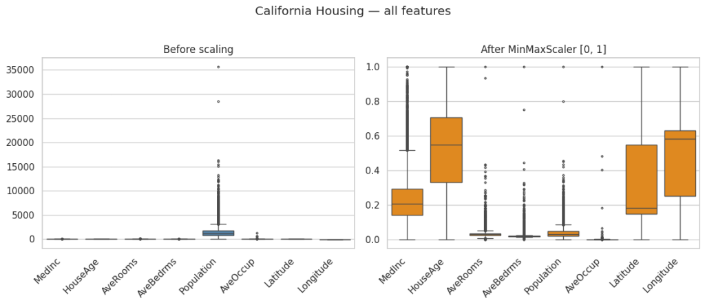
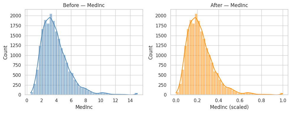
Takeaway: every feature is rescaled to the same [0, 1] range.
  x_scaled = (x - column_min) / (column_max - column_min)

Cheers!