Regularized Regression Techniques: Lasso, Ridge, and Elastic Net
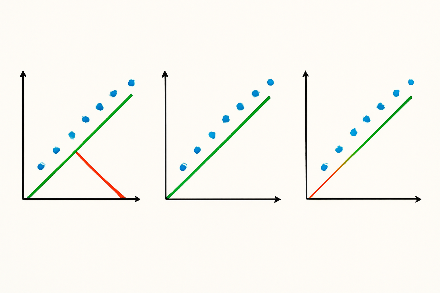
Regularized regression methods are essential tools in machine learning and statistics that help prevent overfitting and improve model generalization by adding penalty terms to the standard linear regression cost function. These techniques are particularly valuable when dealing with high-dimensional data or when the number of features approaches or exceeds the number of observations.
Ridge regression, also known as L2 regularization, adds a penalty term proportional to the sum of squared coefficients to the ordinary least squares (OLS) cost function. This method shrinks the regression coefficients toward zero but never makes them exactly zero.
Ridge Regression ( L2 )
Objective
minimize: Σ ( yᵢ − ŷᵢ )² + λ · Σ βⱼ²
-
ŷᵢ = β₀ + Σ βⱼ xᵢⱼ
-
λ ≥ 0 controls the amount of shrinkage
-
All predictors stay in the model, but coefficients are pulled toward 0.
Lasso Regression ( L1 )
Lasso regression (Least Absolute Shrinkage and Selection Operator) uses L1 regularization, adding a penalty term proportional to the sum of absolute values of coefficients. Unlike Ridge regression, Lasso can drive coefficients to exactly zero, effectively performing feature selection.
Objective
minimize: Σ ( yᵢ − ŷᵢ )² + λ · Σ |βⱼ|
-
Same ŷᵢ and λ as above
-
The absolute-value penalty can push some βⱼ exactly to 0, giving automatic feature selection.
Elastic Net ( L1 + L2 )
Elastic Net regression combines both L1 and L2 penalties, leveraging the strengths of both Ridge and Lasso regression methods. This hybrid approach is particularly effective when dealing with groups of correlated features.
Objective
minimize: Σ ( yᵢ − ŷᵢ )² + λ · [ α · Σ |βⱼ| + (1 − α) · Σ βⱼ² ]
-
0 ≤ α ≤ 1 mixes the two penalties
– α = 1 → pure Lasso
– α = 0 → pure Ridge -
Balances variable selection (L1) with coefficient shrinkage (L2), handling groups of correlated features well.
How to choose
-
Ridge – keep all features, tame multicollinearity.
-
Lasso – need a sparse, easily interpretable model.
-
Elastic Net – expect correlated predictors or want a middle ground.
Tune λ (and α for Elastic Net) with cross-validation for best performance.
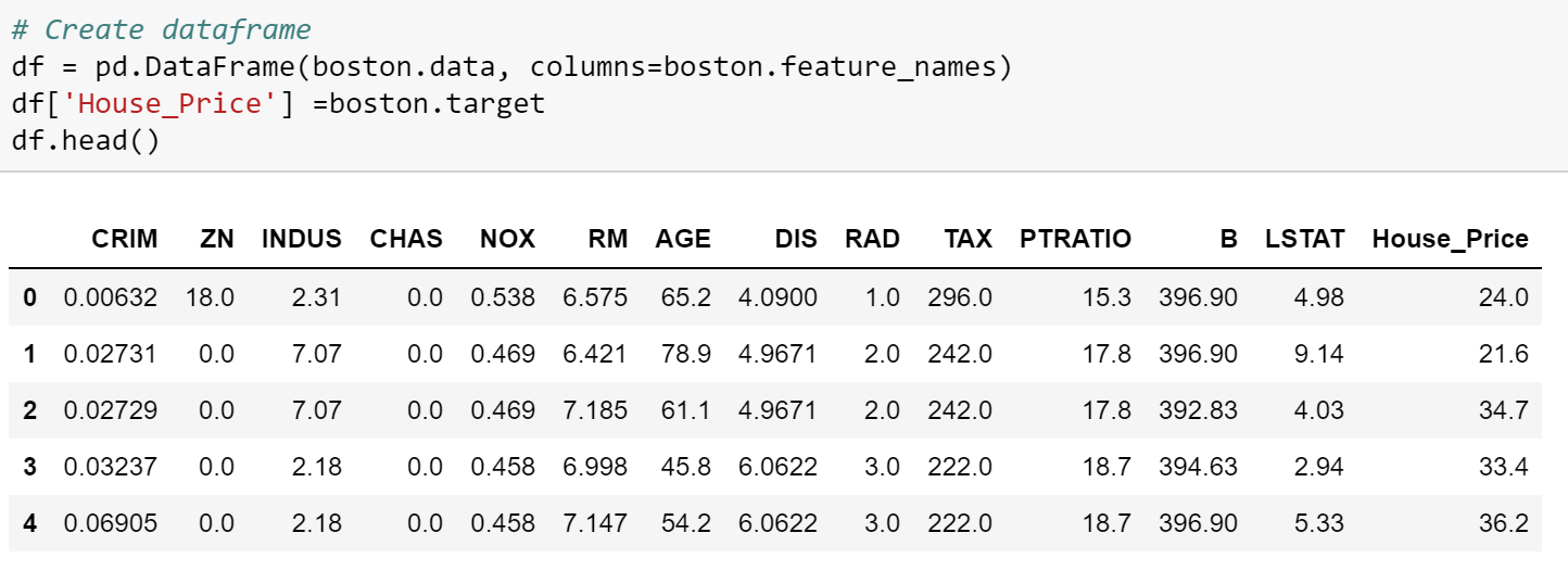
Here is a working example code on the Housing data. Please note, generally before doing regularized GLM regression it is advised to scale variables. However, in the below example we are working with the variables on the original scale to demonstrate each algorithms working.
# Import necessary libraries
from sklearn.linear_model import LinearRegression, Lasso, Ridge, ElasticNet
from sklearn.model_selection import GridSearchCV, train_test_split
from sklearn.metrics import mean_squared_error, mean_absolute_error, r2_score
from sklearn.datasets import fetch_california_housing
from sklearn.preprocessing import StandardScaler
import pandas as pd
import numpy as np
import matplotlib.pyplot as plt
import seaborn as sns
# Load the California Housing dataset
data = fetch_california_housing(as_frame=True)
df = data.frame
# Preprocess the data
X = df.drop(columns=['MedHouseVal'])
y = df['MedHouseVal']
scaler = StandardScaler()
X_scaled = scaler.fit_transform(X)
# Split the data into training and testing sets
X_train, X_test, y_train, y_test = train_test_split(X_scaled, y, test_size=0.2, random_state=42)
# Fit Linear Regression model
linear_model = LinearRegression()
linear_model.fit(X_train, y_train)
y_pred_linear = linear_model.predict(X_test)
# Fit Lasso Regression model with hyperparameter tuning
lasso_params = {'alpha': [0.01, 0.1, 1, 10, 100]}
lasso_model = GridSearchCV(Lasso(), lasso_params, cv=5, scoring='r2')
lasso_model.fit(X_train, y_train)
y_pred_lasso = lasso_model.best_estimator_.predict(X_test)
# Fit Ridge Regression model with hyperparameter tuning
ridge_params = {'alpha': [0.01, 0.1, 1, 10, 100]}
ridge_model = GridSearchCV(Ridge(), ridge_params, cv=5, scoring='r2')
ridge_model.fit(X_train, y_train)
y_pred_ridge = ridge_model.best_estimator_.predict(X_test)
# Fit Elastic Net Regression model with hyperparameter tuning
elastic_params = {'alpha': [0.01, 0.1, 1, 10, 100], 'l1_ratio': [0.1, 0.5, 0.9]}
elastic_model = GridSearchCV(ElasticNet(), elastic_params, cv=5, scoring='r2')
elastic_model.fit(X_train, y_train)
y_pred_elastic = elastic_model.best_estimator_.predict(X_test)
# Evaluate models
results = pd.DataFrame({
'Model': ['Linear', 'Lasso', 'Ridge', 'Elastic Net'],
'MSE': [mean_squared_error(y_test, y_pred_linear),
mean_squared_error(y_test, y_pred_lasso),
mean_squared_error(y_test, y_pred_ridge),
mean_squared_error(y_test, y_pred_elastic)],
'MAE': [mean_absolute_error(y_test, y_pred_linear),
mean_absolute_error(y_test, y_pred_lasso),
mean_absolute_error(y_test, y_pred_ridge),
mean_absolute_error(y_test, y_pred_elastic)],
'R²': [r2_score(y_test, y_pred_linear),
r2_score(y_test, y_pred_lasso),
r2_score(y_test, y_pred_ridge),
r2_score(y_test, y_pred_elastic)]
})
print(results)
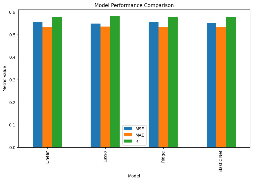
# Plot model performance
results.set_index('Model').plot(kind='bar', figsize=(10, 6))
plt.title('Model Performance Comparison')
plt.ylabel('Metric Value')
plt.show()
# Display coefficients for each model
coefficients = pd.DataFrame({
'Feature': data.feature_names,
'Linear': linear_model.coef_,
'Lasso': lasso_model.best_estimator_.coef_,
'Ridge': ridge_model.best_estimator_.coef_,
'Elastic Net': elastic_model.best_estimator_.coef_
})
print(coefficients)
# Plot coefficients
coefficients.set_index('Feature').plot(kind='bar', figsize=(12, 8))
plt.title('Feature Coefficients for Each Model')
plt.ylabel('Coefficient Value')
plt.show()


You must be logged in to post a comment.