Recommender Engines using Sklearn-Surprise in Python

via GIPHY

What is a Recommendation Engine?

Recommendation engines or systems are machine learning algorithms to make relevant recommendations about the products and services and they are all around us. Few common examples are-

  • Amazon- People who buy this also buy this or who viewed this also viewed this
  • Facebook- Friends recommendation
  • Linkedin- Jobs that match you or network recommendation or who viewed this profile also viewed this profile
  • Netflix- Movies recommendation
  • Google- news recommendation, youtube videos recommendation

Why do we have Recommendation Engines?

The main objective of these recommendation systems is to do following-

  • Customization or personalizaiton
  • Cross sell
  • Up sell
  • Customer retention
  • Address the “Long Tail” phenomenon seen in Online stores vs Brick and Mortar stores

60% of video watch time on Youtube is driven by the recommendation engine.

-Google.com

How do we build a Recommendation Engine?

There are three main approaches for building any recommendation system-

  • Collaborative Filtering

Users and items matrix is built. Normally this matrix is sparse, i.e. most of the cells will be empty and hence some sort of matrix factorization ( such as SVD) is used to reduce dimensions. More on matrix factorization will be discussed later in this article.

The goal of these recommendation system is to find similarities among the users and items and recommend items which have high probability of being liked by a user given the similarities between users and items.

Similarities between users and items embeddings can be assessed using several similarity measures such as Correlation, Cosine Similarities, Jaccard Index, Hamming Distance. The most commonly used similarity measures are dotproducts, Cosine Similarity and Jaccard Index in a recommendation engine

These algorithms don’t require any domain expertise (unlike Content Based models) as it requires only a user and item matrix and related ratings/feedback and hence these algorithms can make a recommendation about an item to a user as long it can identify similar users and item in the matrix .

The flip side of these algorithms is that they may not be suitable for making recommendations about a new item that was not there in the user / item matrix on which the model was trained.

  • Content Based-

This type of recommendation engine focuses on finding characteristics, attributes, tags or features of the items and recommend other items which have some of the same features. Such as, recommend another action movie to a viewer who likes action movies.

Since this algorithm uses features of a product or service to make recommendations, this offers advantage of referring unique or niche items and can be scaled to make recommendations for a wide array of users. On the other hand, defining product features accurately will be key to success of these algorithms.

  • Hybrid- 

These recommendation systems combine both of the above approaches.

Read more here

Build Recommendation System in Python using ” Scikit – Surprise”-

Now let’s switch gears and see how we can build recommendation engines in Python using a special Python library called Surprise. In this exercise, we will build a Collaborative Filtering algorithm using Singular Value Decomposition (SVD) for dimension reduction of a large User-Item Sparse matrix to provide more robust recommendations while avoiding computational complexity.

Here is how you can get started

c1
c2

Please note that if you don’t do the Step 2 correctly, you will get errors such as shown below – ” Failed building wheel for Scikit-surprise” or ” Microsoft Visual C++ 14 is required”

  • Step 3- Install Scikit- Surprise. Please make sure that you have Numpy installed before this

pip install numpy

pip install scikit-surprise

  • Step 4- Import scikit-surprise and make sure it’s correctly loaded

For sake of simplicity, you can also use Google Colab to work on the below example-

Let’s import Movielens small dataset for the purpose of building couple of Recommendation Engines using KNN and SVD algorithms. Please note the that the Surprise package offers many- many more algorithms to choose from. Data can be found at the link-https://grouplens.org/datasets/movielens/

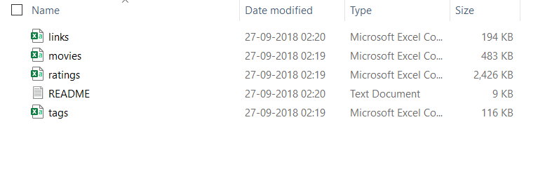
Download the zip files and you will see the following files that you can import in Python to explore. However, for the purpose of CF models, we only need the ratings.csv file.

Here are some key steps that we will follow to build Recommendation Engine for this data

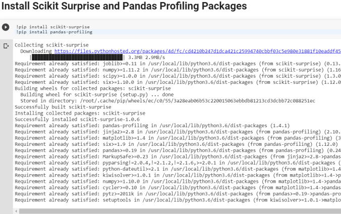
  • Install Scikit Surprise and Pandas Profiling Packages
  • Import necessary packages
  • Type Magic command to print multiple statements on a same line
  • Import all files to explore data
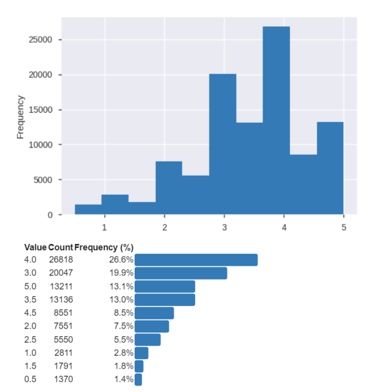
  • Explore datasets using Pandas Profiling Package
  • Use Reader class to parse the file correctly for Surprise package to read and process the file
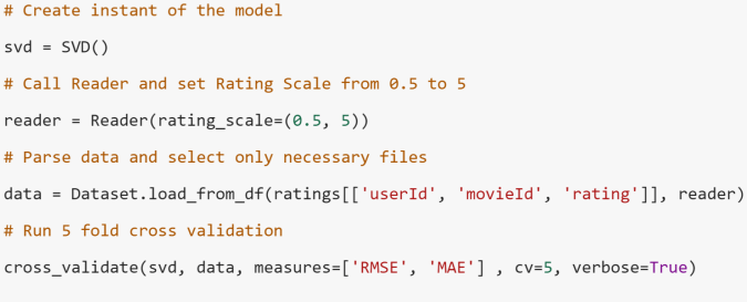
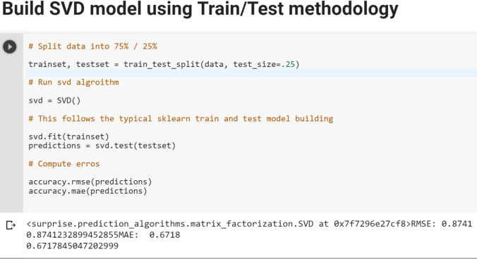
  • Build SVD model using cross-validation methodology
  • Build SVD model using Train/Test methodology
  • Make predictions of Ratings for a particular user and movie
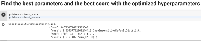
  • Build KNN based Recommender and optimize hyperparameters using Gridsearch
  • Find the best parameters and the best score with the optimized hyperparameters

Below are some other useful links from the Surprise Package.

Examples

Getting Started

Movie Example

Finally, here is a paper on Amazon Recommendation Engine.

Cheers!

Market Basket Analysis or Association Rules or Affinity Analysis or Apriori Algorithm

First of all, if you are not familiar with the concept of Market Basket Analysis (MBA), Association Rules or Affinity Analysis and related metrics such as Support, Confidence and Lift, please read this article first.

Here is how we can do it in Python. We will look at two examples-

Example 1-

Data used for this example can be found here Retail_Data.csv

mba1mba2mba3

Example 2-

MBA4MBA5MBA6

Cheers!

Linear Discriminant Analysis ( LDA) with Scikit

Linear Discriminant Analysis (LDA) is similar to Principal Component Analysis (PCA) in reducing the dimensionality. However, there are certain nuances with LDA that we should be aware of-

  • LDA is supervised (needs categorical dependent variable) to provide the best linear combination of original variables while providing the maximum separation among the different groups. On the other hand, PCA is unsupervised
  • LDA can be used for classification also, whereas PCA is generally used for unsupervised learning
  • LDA doesn’t need the numbers of discriminant to be passed on ahead of time. Generally speaking the number of discriminant will be lower of the number of variables or number of categories-1.
  • LDA is more robust and can be conducted without even standardizing or normalizing the variables in certain cases
  • LDA is preferred for bigger data sets and machine learning

Let the action begin now-

lda1LDA2LDA3LDA4LDA5

Cheers!

Principal Component Analysis ( PCA) using Scikit

Principal Component Analysis ( PCA) is generally used as an unsupervised algorithm for reducing the data dimensions to address Curse of Dimensionality, detecting outliers, removing noise, speech recognition and other such areas.

The underlying algorithm in PCA is generally a linear algebra technique called Singular Value Decomposition (SVD). PCAs take the original data and create orthogonal components (uncorrelated components) that capture the information contained in the original data however with significantly less number of components.

Either the components themselves or  key loading of the components can be plugged in any further modeling work, rather than the original data to minimize information redundancy and noise.

There are three main ways to select the right number of components-

  1. Number of components should explain at least 80% of the original data variance or information [Preferred One]
  2. Eigen value of each PCA component should be more than or equal to 1. This means that they should express at least one variable worth of information
  3. Elbow or Scree method- look for the elbow in the percentage of variance explained by each components and select the components where an elbow or kink is visible.

You can use any one of the above or combination of the above to select the right number of components. It is very critical to standardize or normalize data before conducting PCA.

In the below case study we will use the first criterion shown above, i.e. 80% or more of the original data variance should be explained by the selected number of components.

PCA1PCA2PCA3PCA4PCA5PCA6

Logistic Regression using Scikit Python

If you are not familiar with logistics regression, please read this article first. Moreover, if you are not familiar with the sklearn machine learning model building process, please read this article also.

Assuming you are now familiar, this is how you can build a logistic regression model in Python using machine learning library Scikit.  Please read here about the dataset and dummy coding. 

clf1clf2clf3clf4clf5clf6clf7

clf8clf9clf10

Cheers!

Categorical Variables Dummy Coding

Converting categorical variables into numerical dummy coded variable is generally a requirement in machine learning libraries such as Scikit as they mostly work on numpy arrays.

In this blog, let’s look at how we can convert bunch of categorical variables into numerical dummy coded variables using four different methods-

  1. Scikit learn preprocessing LabelEncoder
  2.  Pandas getdummies
  3. Looping
  4. Mapping

We will work with a dataset from IBM Watson blog as this has plenty of categorical variables. You can find the data here.  In this data, we are trying to build a model to predict “churn”, which has two levels “Yes” and “No”.

We will convert the dependent variable using Scikit LabelEncoder and the independent categorical variables using Pandas getdummies. Please note that LabelEncoder will not necessarily create additional columns, whereas the getdummies will create additional columns in the data. We will see that in the below example-

clf1clf2clf3clf4clf5clf6clf7

Here are few other ways to dummy coding-

dummy_coding1dummy_coding2dummy_coding3

Here is an excellent Kaggle Kernel for detailed feature engineering.

Cheers!

Hierarchical Clustering with Python

As highlighted in the article, clustering and segmentation play an instrumental role in Data Science. In this blog, we will show you how to build a Hierarchical Clustering with Python.

For this purpose, we will work with a R dataset called “Cheese”. Please install package called “Bayesm” in R and export this data set in csv format to be imported in Python. More on this dataset can be found here.

Let’s begin with the clustering in Python then. hclust1hclust2hclust3hclust4hclust5hclust6hclust7

hclust8

Cheers!

KMeans Clustering: Core Concepts, Assumptions, and Key Equations

Overview:
KMeans is an unsupervised machine learning algorithm used to partition data into a specified number of clusters (k). Each cluster is defined by its centroid, and the algorithm aims to minimize the distance between data points and their assigned cluster centroids.

Core Concepts:

  1. Clusters and Centroids:

    • A cluster is a group of data points that are similar to each other.
    • The centroid is the mean position of all the points in a cluster.
  2. Assignment and Update Steps:

    • Assignment: Each data point is assigned to the nearest centroid.
    • Update: The centroids are recalculated as the mean of all points assigned to each cluster.
  3. Iterative Optimization:

    • The assignment and update steps are repeated until the centroids no longer change significantly or a maximum number of iterations is reached.

Assumptions:

  • The number of clusters (k) is known and fixed in advance.
  • Clusters are roughly spherical and equally sized.
  • Data points are closer to their own cluster centroid than to others.
  • The algorithm is sensitive to the initial placement of centroids.

Key Equations:

  1. Distance Calculation:

    • The most common distance metric is Euclidean distance.
    • For a data point x and centroid c:
      Distance = sqrt( (x1 – c1)^2 + (x2 – c2)^2 + … + (xn – cn)^2 )
  2. Centroid Update:

    • For each cluster, the new centroid is the mean of all points assigned to that cluster.
    • Centroid for cluster j:
      cj = (1 / Nj) * sum(xi)
      where Nj is the number of points in cluster j, and xi are the points in cluster j.
  3. Objective Function (Inertia):

    • KMeans minimizes the sum of squared distances (inertia) between each point and its assigned centroid.
    • Inertia = sum over all clusters j [ sum over all points i in cluster j (distance(xi, cj))^2 ]

Algorithm Steps:

  1. Choose k initial centroids (randomly or using a method like k-means++).
  2. Assign each data point to the nearest centroid.
  3. Recalculate centroids as the mean of assigned points.
  4. Repeat steps 2 and 3 until centroids stabilize.

Limitations:

  • Sensitive to outliers and noise.
  • May converge to a local minimum (results can vary with different initializations).
  • Not suitable for clusters with non-spherical shapes or very different sizes.

Applications:

  • Market segmentation
  • Image compression
  • Document clustering
  • Anomaly detection

# Simple KMeans Clustering Example
import numpy as np
import matplotlib.pyplot as plt
from sklearn.datasets import make_blobs
from sklearn.cluster import KMeans
from sklearn.metrics import silhouette_score

# Generate synthetic data
X, y_true = make_blobs(n_samples=300, centers=4, cluster_std=0.60, random_state=42)

# Elbow method to find optimal k
inertia = []
k_range = range(1, 11)
for k in k_range:
    kmeans = KMeans(n_clusters=k, random_state=42)
    kmeans.fit(X)
    inertia.append(kmeans.inertia_)
plt.figure(figsize=(6,4))
plt.plot(k_range, inertia, 'bo-')
plt.axvline(x=4, color='red', linestyle='--', label='Optimal k=4')
plt.xlabel('Number of clusters (k)')
plt.ylabel('Inertia')
plt.title('Elbow Method for Optimal k')
plt.legend()
plt.grid(True)
plt.show()

# Fit KMeans with optimal k (choose visually, e.g., k=4)
k_opt = 4
kmeans = KMeans(n_clusters=k_opt, random_state=42)
labels = kmeans.fit_predict(X)

# Plot clusters
plt.figure(figsize=(7,5))
plt.scatter(X[:, 0], X[:, 1], c=labels, cmap='viridis', s=50)
plt.scatter(kmeans.cluster_centers_[:, 0], kmeans.cluster_centers_[:, 1], c='red', s=200, alpha=0.75, marker='X', label='Centers')
plt.title(f'KMeans Clustering (k={k_opt})')
plt.xlabel('Feature 1')
plt.ylabel('Feature 2')
plt.legend()
plt.show()

# Silhouette score
score = silhouette_score(X, labels)
print(f'Silhouette Score (k={k_opt}): {score:.3f}')

Silhouette Score (k=4): 0.876

# KMeans Clustering on Iris Dataset
import numpy as np
import matplotlib.pyplot as plt
from sklearn.datasets import load_iris
from sklearn.cluster import KMeans
from sklearn.metrics import silhouette_score
import pandas as pd

# Load Iris data
iris = load_iris()
X = iris.data

# Elbow method to find optimal k
inertia = []
k_range = range(1, 11)
for k in k_range:
    kmeans = KMeans(n_clusters=k, random_state=42)
    kmeans.fit(X)
    inertia.append(kmeans.inertia_)
k_opt = 3  # Set optimal k explicitly for Iris data
plt.figure(figsize=(6,4))
plt.plot(k_range, inertia, 'bo-')
plt.axvline(x=k_opt, color='red', linestyle='--', label='Optimal k=3')
plt.xlabel('Number of clusters (k)')
plt.ylabel('Inertia')
plt.title('Elbow Method for Optimal k (Iris)')
plt.legend()
plt.grid(True)
plt.show()

# Fit KMeans with optimal k (choose visually, e.g., k=3)
kmeans = KMeans(n_clusters=k_opt, random_state=42)
labels = kmeans.fit_predict(X)

# Plot clusters (using first two features for visualization)
plt.figure(figsize=(7,5))
plt.scatter(X[:, 0], X[:, 1], c=labels, cmap='viridis', s=50)
plt.scatter(kmeans.cluster_centers_[:, 0], kmeans.cluster_centers_[:, 1], c='red', s=200, alpha=0.75, marker='X', label='Centers')
plt.title(f'Iris KMeans Clustering (k={k_opt})')
plt.xlabel(iris.feature_names[0])
plt.ylabel(iris.feature_names[1])
plt.legend()
plt.show()

# Plot clusters (using petal length and petal width for visualization)
plt.figure(figsize=(7,5))
plt.scatter(X[:, 2], X[:, 3], c=labels, cmap='viridis', s=50)
plt.scatter(kmeans.cluster_centers_[:, 2], kmeans.cluster_centers_[:, 3], c='red', s=200, alpha=0.75, marker='X', label='Centers')
plt.title(f'Iris KMeans Clustering (k={k_opt}) - Petal Length vs Petal Width')
plt.xlabel(iris.feature_names[2])
plt.ylabel(iris.feature_names[3])
plt.legend()
plt.show()

# Silhouette score
score = silhouette_score(X, labels)
print(f'Silhouette Score (k={k_opt}): {score:.3f}')

# Number of observations in each cluster
unique, counts = np.unique(labels, return_counts=True)
for i, count in zip(unique, counts):
    print(f"Cluster {i}: {count} data points")

# Descriptive summary of each cluster (mean feature values)
df = pd.DataFrame(X, columns=iris.feature_names)
df['cluster'] = labels
print("\nCluster feature means:")
print(df.groupby('cluster').mean())

Cheers!