
Overview:
KMeans is an unsupervised machine learning algorithm used to partition data into a specified number of clusters (k). Each cluster is defined by its centroid, and the algorithm aims to minimize the distance between data points and their assigned cluster centroids.
Core Concepts:
-
Clusters and Centroids:
- A cluster is a group of data points that are similar to each other.
- The centroid is the mean position of all the points in a cluster.
-
Assignment and Update Steps:
- Assignment: Each data point is assigned to the nearest centroid.
- Update: The centroids are recalculated as the mean of all points assigned to each cluster.
-
Iterative Optimization:
- The assignment and update steps are repeated until the centroids no longer change significantly or a maximum number of iterations is reached.
Assumptions:
- The number of clusters (k) is known and fixed in advance.
- Clusters are roughly spherical and equally sized.
- Data points are closer to their own cluster centroid than to others.
- The algorithm is sensitive to the initial placement of centroids.
Key Equations:
-
Distance Calculation:
- The most common distance metric is Euclidean distance.
- For a data point x and centroid c:
Distance = sqrt( (x1 – c1)^2 + (x2 – c2)^2 + … + (xn – cn)^2 )
-
Centroid Update:
- For each cluster, the new centroid is the mean of all points assigned to that cluster.
- Centroid for cluster j:
cj = (1 / Nj) * sum(xi)
where Nj is the number of points in cluster j, and xi are the points in cluster j.
-
Objective Function (Inertia):
- KMeans minimizes the sum of squared distances (inertia) between each point and its assigned centroid.
- Inertia = sum over all clusters j [ sum over all points i in cluster j (distance(xi, cj))^2 ]
Algorithm Steps:
- Choose k initial centroids (randomly or using a method like k-means++).
- Assign each data point to the nearest centroid.
- Recalculate centroids as the mean of assigned points.
- Repeat steps 2 and 3 until centroids stabilize.
Limitations:
- Sensitive to outliers and noise.
- May converge to a local minimum (results can vary with different initializations).
- Not suitable for clusters with non-spherical shapes or very different sizes.
Applications:
- Market segmentation
- Image compression
- Document clustering
- Anomaly detection
# Simple KMeans Clustering Example
import numpy as np
import matplotlib.pyplot as plt
from sklearn.datasets import make_blobs
from sklearn.cluster import KMeans
from sklearn.metrics import silhouette_score

# Generate synthetic data
X, y_true = make_blobs(n_samples=300, centers=4, cluster_std=0.60, random_state=42)

# Elbow method to find optimal k
inertia = []
k_range = range(1, 11)
for k in k_range:
    kmeans = KMeans(n_clusters=k, random_state=42)
    kmeans.fit(X)
    inertia.append(kmeans.inertia_)
plt.figure(figsize=(6,4))
plt.plot(k_range, inertia, 'bo-')
plt.axvline(x=4, color='red', linestyle='--', label='Optimal k=4')
plt.xlabel('Number of clusters (k)')
plt.ylabel('Inertia')
plt.title('Elbow Method for Optimal k')
plt.legend()
plt.grid(True)
plt.show()

# Fit KMeans with optimal k (choose visually, e.g., k=4)
k_opt = 4
kmeans = KMeans(n_clusters=k_opt, random_state=42)
labels = kmeans.fit_predict(X)

# Plot clusters
plt.figure(figsize=(7,5))
plt.scatter(X[:, 0], X[:, 1], c=labels, cmap='viridis', s=50)
plt.scatter(kmeans.cluster_centers_[:, 0], kmeans.cluster_centers_[:, 1], c='red', s=200, alpha=0.75, marker='X', label='Centers')
plt.title(f'KMeans Clustering (k={k_opt})')
plt.xlabel('Feature 1')
plt.ylabel('Feature 2')
plt.legend()
plt.show()

# Silhouette score
score = silhouette_score(X, labels)
print(f'Silhouette Score (k={k_opt}): {score:.3f}')

Silhouette Score (k=4): 0.876
# KMeans Clustering on Iris Dataset
import numpy as np
import matplotlib.pyplot as plt
from sklearn.datasets import load_iris
from sklearn.cluster import KMeans
from sklearn.metrics import silhouette_score
import pandas as pd
# Load Iris data
iris = load_iris()
X = iris.data
# Elbow method to find optimal k
inertia = []
k_range = range(1, 11)
for k in k_range:
kmeans = KMeans(n_clusters=k, random_state=42)
kmeans.fit(X)
inertia.append(kmeans.inertia_)
k_opt = 3 # Set optimal k explicitly for Iris data
plt.figure(figsize=(6,4))
plt.plot(k_range, inertia, 'bo-')
plt.axvline(x=k_opt, color='red', linestyle='--', label='Optimal k=3')
plt.xlabel('Number of clusters (k)')
plt.ylabel('Inertia')
plt.title('Elbow Method for Optimal k (Iris)')
plt.legend()
plt.grid(True)
plt.show()
# Fit KMeans with optimal k (choose visually, e.g., k=3)
kmeans = KMeans(n_clusters=k_opt, random_state=42)
labels = kmeans.fit_predict(X)
# Plot clusters (using first two features for visualization)
plt.figure(figsize=(7,5))
plt.scatter(X[:, 0], X[:, 1], c=labels, cmap='viridis', s=50)
plt.scatter(kmeans.cluster_centers_[:, 0], kmeans.cluster_centers_[:, 1], c='red', s=200, alpha=0.75, marker='X', label='Centers')
plt.title(f'Iris KMeans Clustering (k={k_opt})')
plt.xlabel(iris.feature_names[0])
plt.ylabel(iris.feature_names[1])
plt.legend()
plt.show()
# Plot clusters (using petal length and petal width for visualization)
plt.figure(figsize=(7,5))
plt.scatter(X[:, 2], X[:, 3], c=labels, cmap='viridis', s=50)
plt.scatter(kmeans.cluster_centers_[:, 2], kmeans.cluster_centers_[:, 3], c='red', s=200, alpha=0.75, marker='X', label='Centers')
plt.title(f'Iris KMeans Clustering (k={k_opt}) - Petal Length vs Petal Width')
plt.xlabel(iris.feature_names[2])
plt.ylabel(iris.feature_names[3])
plt.legend()
plt.show()
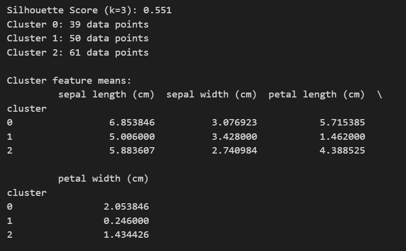
# Silhouette score
score = silhouette_score(X, labels)
print(f'Silhouette Score (k={k_opt}): {score:.3f}')
# Number of observations in each cluster
unique, counts = np.unique(labels, return_counts=True)
for i, count in zip(unique, counts):
print(f"Cluster {i}: {count} data points")
# Descriptive summary of each cluster (mean feature values)
df = pd.DataFrame(X, columns=iris.feature_names)
df['cluster'] = labels
print("\nCluster feature means:")
print(df.groupby('cluster').mean())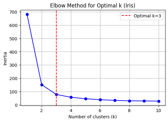


Cheers!

Pingback: Learn Python Step by Step | RP's Blog on data science
Please share the link to download cheese dataset
LikeLike
Hi Sumit: Cheese data is part of the R package called ” Bayesm” . Here is the link- https://rdrr.io/cran/bayesm/man/cheese.html
LikeLike