Recurrent Neural Network (RNN) are a special type of feed-forward network used for sequential data analysis where inputs are not independent and are not of fixed length as is assumed in some of the other neural networks such as MLP. Rather in this case, inputs are dependent on each other along the time dimension. In other words, what happens in time ‘t’ may depend on what happened in time ‘t-1’, ‘t-2’ and so on.
These are also called ‘memory’ networks as previous inputs and states persist in the model for doing a more optimal sequential analysis. They can have both short term and long term time dependence. Due to their capabilities of handling sequential data very well, these networks are typically very suitable for speech recognition, sentiment analysis, forecasting, language translation and other such applications.
Let’s now spend sometime looking at how a RNN work-
Recurrent Neural Network (RNN)
As you may recall, in a typical feed-forward neural network input is fed at beginning and then hidden layers do the processing and finally output layer spits out the output. On the other hand, in a RNN generally speaking we will have different input, output and cost function for each time stamp. However, the same weight matrix is fed to all layers in the network.
One point to note is that RNNs are also trained using backward propagation of errors and gradient descent to minimize cost function. However, backward propagation in RNN happen over different time stamps and hence it’s called Backward Propagation Through Time (BPTT). In a typical RNN, we may have several time stamp layers which sometimes may range in hundreds or thousands and therein lies the problem of vanishing gradient or exploding gradient that these pure vanilla RNNs are particularly susceptible for.
There are various techniques such as gradient clipping and architecture such as Long Short Term Memory (LSTM) or Gated Recurrent Unit (GRU) which help in fixing the vanishing gradient and exploding gradient issues. We will delve deeper into how an LSTM work.
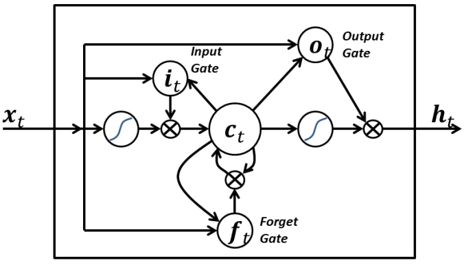
A LSTM network consist of hidden layers that have many LSTM blocks or units. In turn each LSTM unit will have the following components-
Memory Cell- The component that remembers the values over a period of time. This has an activation function
Input gate- Enables addition of info to the memory cell. Generally has as an tanh activation to squash the values between -1 and +1
Forget gate- Enables removing or retaining from the memory cell. This will generally have a sigmoid activation function and hence the output values will range between 0 and 1. If the gate is on, then all memories are retained. If the gate is turned-off, all values will be removed.
Output gate- Retrieve information from the memory cell passed through the tanh activation
Long Short Term Memory Cell or Block (Source- Wiki)
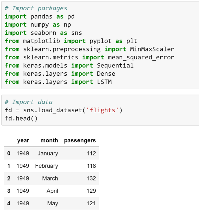
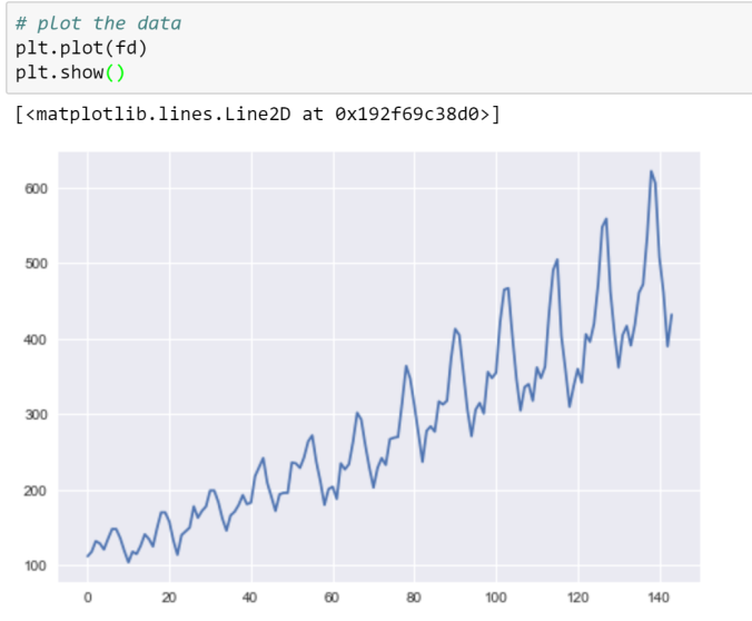
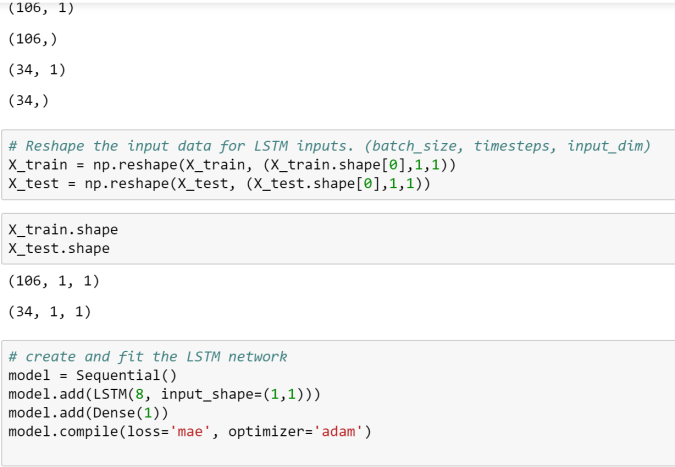
Let’s work through an example which we used in a previous article.
Here is an excellent article in case you want to explore more.
Ensemble models are a great tool to fix the variance-bias trade-off which a typical machine learning model faces, i.e. when you try to lower bias, variance will go higher and vice-versa. This generally results in higher error rates.
Total Error in Model = Bias + Variance + Random Noise
Variance and Bias Trade-off
Ensemble models typically combine several weak learners to build a stronger model, which will reduce variance and bias at the same time. Since ensemble models follow a community learning or divide and conquer approach, output from ensemble models will be wrong only when the majority of underlying learners are wrong.
One of the biggest flip side of ensemble models is that they may become “Black Box” and not very explainable as opposed a simple machine learning model. However, the gains in model performances generally outweigh any loss in transparency. That is the reason why you will see top performing models in many high ranking competitions will be generally an ensemble model.
Ensemble models can be broken down into the following three main categories-
Bagging
Boosting
Stacking
Let’s look at each one of them-
Bagging-
One good example of such model is Random Forest
These types of ensemble models work on reducing the variance by removing instability in the underlying complex models
Each learner is asked to do the classification or regression independently and in parallel and then either a voting or averaging of the output of all the learners is done to create the final output
Since these ensemble models are predominantly focuses on reducing the variance, the underlying models are fairly complex ( such as Decision Tree or Neural Network) to begin with low bias
An underlying decision tree will have higher depth and many branches. In other words, the tree will be deep and dense and with lower bias
Boosting-
Some good examples of these types of models are Gradient Boosting Tree, Adaboost, XGboost among others.
These ensemble models work with weak learners and try to improve the bias and variance simultaneously by working sequentially.
These are also called adaptive learners, as learning of one learner is dependent on how other learners are performing. For example, if a certain set of the data has higher mis-classification rate, this sample’s weight in the overall learning will be increased so that the other learners focus more on correctly classifying the tougher samples.
An underlying decision tree will be shallow and a weak learner with higher bias
There are various approaches for building a bagging model such as- pasting, bagging, random subspaces, random patches etc. You can find all details over here.
Stacking-
These meta learning models are what the name suggest. They are stacked models. Or in other words, a particular learner’s output will become an input to another model and so on.
Random Forest: Comprehensive Explanation
Core Concepts
Random Forest is an ensemble learning method that combines multiple decision trees to create a more robust and accurate predictive model. The algorithm works by building numerous decision trees and merging their predictions through voting (for classification) or averaging (for regression).
Key Principles
Bootstrap Aggregating (Bagging): Each tree in the forest is trained on a different bootstrap sample of the original dataset. This means each tree sees a slightly different version of the data, created by randomly sampling with replacement.
Feature Randomness: At each split in each tree, only a random subset of features is considered. This introduces additional randomness and helps prevent overfitting while reducing correlation between trees.
Ensemble Voting: For classification, each tree votes for a class, and the class with the most votes becomes the final prediction. For regression, predictions are averaged across all trees.
Core Assumptions
Independence of Errors: Individual trees should make different types of errors so that when combined, these errors cancel out
Feature Relevance: The dataset should contain features that are actually predictive of the target variable
Sufficient Data: There should be enough data to train multiple diverse trees effectively
Non-linear Relationships: Random forests can capture complex, non-linear relationships between features and targets
Key Equations and Formulas
Bootstrap Sample Size: Each bootstrap sample typically contains the same number of observations as the original dataset (n), created by sampling with replacement.
Number of Features at Each Split: For classification: sqrt(total_features), for regression: total_features/3
Final Prediction for Classification: Prediction = mode(tree1_prediction, tree2_prediction, …, treeN_prediction)
Final Prediction for Regression: Prediction = (tree1_prediction + tree2_prediction + … + treeN_prediction) / N
Out-of-Bag (OOB) Error: Each tree is tested on the ~37% of samples not included in its bootstrap sample, providing an unbiased estimate of model performance without needing a separate validation set.
Variable Importance: Calculated by measuring how much each feature decreases impurity when used for splits, averaged across all trees in the forest.
Advantages
Reduced Overfitting: Ensemble approach generalizes better than individual decision trees
Handles Missing Values: Can maintain accuracy even with missing data
No Feature Scaling Required: Tree-based methods are not affected by feature scaling
Robust to Outliers: Tree splits are not heavily influenced by extreme values
End to End Python Execution-
# - Random Forest Regression on California Housing Dataset
# - RandomizedSearchCV vs GridSearchCV:
# - GridSearchCV exhaustively tries every combination of hyperparameters in the provided grid.
# - RandomizedSearchCV samples a fixed number of random combinations from the grid, making it faster for large search spaces.
# - Both are used for hyperparameter optimization, but RandomizedSearchCV is more efficient when the grid is large or when you want a quick search.
import numpy as np # For numerical operations
import pandas as pd # For data manipulation
import matplotlib.pyplot as plt # For plotting
import seaborn as sns # For advanced visualizations
from sklearn.datasets import fetch_california_housing # To load the dataset
from sklearn.model_selection import train_test_split, GridSearchCV, RandomizedSearchCV # For splitting and hyperparameter search
from sklearn.ensemble import RandomForestRegressor # Random Forest regression model
from sklearn.metrics import mean_squared_error, r2_score # For regression metrics
import warnings # To suppress warnings
warnings.filterwarnings('ignore') # Ignore warnings for cleaner output
# Load California housing dataset
cal_data = fetch_california_housing() # Fetch the dataset
X = pd.DataFrame(cal_data.data, columns=cal_data.feature_names) # Features as DataFrame
y = cal_data.target # Target variable (median house value)
# Train-test split
X_train, X_test, y_train, y_test = train_test_split(X, y, test_size=0.3, random_state=42) # Split data into train and test sets
# Fixed lists for hyperparameters
param_list = {
'n_estimators': [50, 100, 150, 200], # Number of trees in the forest
'max_depth': [5, 10, 15, None], # Maximum depth of the tree
'min_samples_split': [2, 4, 6, 8], # Minimum samples required to split a node
'min_samples_leaf': [1, 2, 3], # Minimum samples required at a leaf node
'max_features': ['sqrt', 'log2', None], # Number of features to consider at each split
'bootstrap': [True, False] # Whether bootstrap samples are used
}
# RandomizedSearchCV for Random Forest Regressor
rf = RandomForestRegressor(random_state=42) # Initialize Random Forest Regressor
random_search = RandomizedSearchCV(
rf, param_distributions=param_list, n_iter=20, cv=3, scoring='neg_mean_squared_error', n_jobs=-1, random_state=42) # Randomized hyperparameter search
random_search.fit(X_train, y_train) # Fit model to training data
print('Best parameters (RandomizedSearchCV):', random_search.best_params_) # Print best parameters
print('Best score (RandomizedSearchCV):', -random_search.best_score_) # Print best score (MSE)
rf_random = random_search.best_estimator_ # Get best model
# GridSearchCV for Random Forest Regressor (commented out)
# grid_search = GridSearchCV(
# rf, param_grid=param_list, cv=3, scoring='neg_mean_squared_error', n_jobs=-1) # Grid hyperparameter search
# grid_search.fit(X_train, y_train) # Fit model to training data
# print('Best parameters (GridSearchCV):', grid_search.best_params_) # Print best parameters
# print('Best score (GridSearchCV):', -grid_search.best_score_) # Print best score (MSE)
# rf_grid = grid_search.best_estimator_ # Get best model
# Evaluate RandomizedSearchCV model
y_pred = rf_random.predict(X_test) # Predict on test set
mse = mean_squared_error(y_test, y_pred) # Calculate mean squared error
r2 = r2_score(y_test, y_pred) # Calculate R^2 score
print(f'\nRandomizedSearchCV Test MSE: {mse:.4f}') # Print test MSE
print(f'RandomizedSearchCV Test R2: {r2:.4f}') # Print test R^2
plt.figure(figsize=(6,5)) # Set figure size
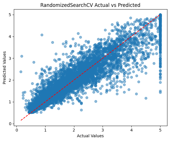
plt.scatter(y_test, y_pred, alpha=0.5) # Scatter plot of actual vs predicted
plt.plot([y_test.min(), y_test.max()], [y_test.min(), y_test.max()], 'r--') # Diagonal reference line
plt.xlabel('Actual Values') # X-axis label
plt.ylabel('Predicted Values') # Y-axis label
plt.title('RandomizedSearchCV Actual vs Predicted') # Plot title
plt.tight_layout() # Adjust layout
plt.show() # Show plot
# Feature importance visualization for best RandomizedSearchCV model
importances = rf_random.feature_importances_ # Get feature importances
indices = np.argsort(importances)[::-1] # Sort features by importance
plt.figure(figsize=(8,5)) # Set figure size
plt.bar(range(X.shape[1]), importances[indices], align='center') # Bar plot of importances
plt.xticks(range(X.shape[1]), [X.columns[i] for i in indices], rotation=45) # Feature names as x-ticks
plt.title('Feature Importances (RandomizedSearchCV Best Model)') # Plot title
plt.tight_layout() # Adjust layout
plt.show() # Show plot
# Visualize a single tree from the Random Forest
from sklearn.tree import plot_tree
plt.figure(figsize=(20,10))
plot_tree(rf_random.estimators_[0], feature_names=X.columns, filled=True, max_depth=2)
plt.title('Random Forest Regression: Example Tree (Depth=2)')
plt.show()
Best parameters (RandomizedSearchCV): {‘n_estimators’: 50, ‘min_samples_split’: 8, ‘min_samples_leaf’: 1, ‘max_features’: ‘log2’, ‘max_depth’: 15, ‘bootstrap’: False} Best score (RandomizedSearchCV): 0.26113711835896053 RandomizedSearchCV Test MSE: 0.2415 RandomizedSearchCV Test R2: 0.8160
# Titanic Classification with Random Forest (Simplified)
import pandas as pd
import numpy as np
from sklearn.ensemble import RandomForestClassifier
from sklearn.model_selection import train_test_split, RandomizedSearchCV
from sklearn.metrics import accuracy_score, confusion_matrix, classification_report
from sklearn.preprocessing import LabelEncoder, StandardScaler
import seaborn as sns
import matplotlib.pyplot as plt
from sklearn.tree import plot_tree
# Load and preprocess Titanic dataset
X = sns.load_dataset('titanic').drop(['survived', 'deck', 'embark_town', 'alive', 'class', 'who'], axis=1)
X['age'] = X['age'].fillna(X['age'].median())
X['fare'] = X['fare'].fillna(X['fare'].median())
X['embarked'] = X['embarked'].fillna(X['embarked'].mode()[0])
X['alone'] = X['alone'].fillna(X['alone'].mode()[0])
for col in ['sex', 'embarked', 'alone']:
X[col] = LabelEncoder().fit_transform(X[col])
X = X.drop(['adult_male'], axis=1)
scaler = StandardScaler()
X_scaled = scaler.fit_transform(X)
y = sns.load_dataset('titanic')['survived']
# Train-test split
X_train, X_test, y_train, y_test = train_test_split(X_scaled, y, test_size=0.3, random_state=42, stratify=y)
# Random Forest with RandomizedSearchCV
rf = RandomForestClassifier(random_state=42)
param_dist = {
'n_estimators': [100, 200, 300],
'max_depth': [5, 10, None],
'min_samples_split': [2, 4, 6],
'min_samples_leaf': [1, 2, 3],
'max_features': ['sqrt', 'log2']
}
random_search = RandomizedSearchCV(rf, param_distributions=param_dist, n_iter=15, cv=3, scoring='accuracy', n_jobs=-1, random_state=42)
random_search.fit(X_train, y_train)
rf_best = random_search.best_estimator_
# Evaluation
y_pred = rf_best.predict(X_test)
print('Test Accuracy:', accuracy_score(y_test, y_pred))
print(classification_report(y_test, y_pred))
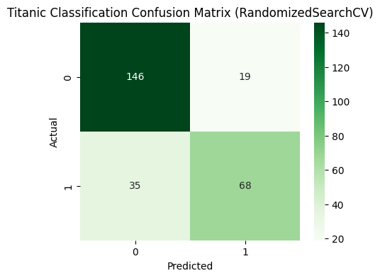
cm = confusion_matrix(y_test, y_pred)
plt.figure(figsize=(5,4))
sns.heatmap(cm, annot=True, fmt='d', cmap='Greens')
plt.title('Titanic Classification Confusion Matrix')
plt.xlabel('Predicted')
plt.ylabel('Actual')
plt.show()
# Feature importance
importances = rf_best.feature_importances_
indices = np.argsort(importances)[::-1]
plt.figure(figsize=(8,5))
plt.bar(range(X.shape[1]), importances[indices], align='center')
plt.xticks(range(X.shape[1]), [X.columns[i] for i in indices], rotation=45)
plt.title('Feature Importances (Titanic Random Forest)')
plt.tight_layout()
plt.show()
# Visualize tree with most important root split
root_feature = indices[0]
tree_idx = next((i for i, est in enumerate(rf_best.estimators_) if est.tree_.feature[0] == root_feature), 0)
plt.figure(figsize=(20,10))
plot_tree(rf_best.estimators_[tree_idx], feature_names=X.columns, filled=True, max_depth=2)
plt.title(f'Titanic Random Forest: Example Tree (Root={X.columns[root_feature]})')
plt.show()
Best parameters (RandomizedSearchCV): {‘n_estimators’: 200, ‘min_samples_split’: 2, ‘min_samples_leaf’: 1, ‘max_features’: ‘sqrt’, ‘max_depth’: 10} Best cross-validated accuracy (RandomizedSearchCV): 0.8378700606961477 Test Accuracy (RandomizedSearchCV): 0.7985074626865671
Convolution Neural Network (CNN) are particularly useful for spatial data analysis, image recognition, computer vision, natural language processing, signal processing and variety of other different purposes. They are biologically motivated by functioning of neurons in visual cortex to a visual stimuli.
What makes CNN much more powerful compared to the other feedback forward networks for image recognition is the fact that they do not require as much human intervention and parameters as some of the other networks such as MLP do. This is primarily driven by the fact that CNNs have neurons arranged in three dimensions.
CNNs make all of this magic happen by taking a set of input and passing it on to one or more of following main hidden layers in a network to generate an output.
Let’s dig deeper into utility of each of the above layers.
Convolution Layers– Before we move this discussion any further, let’s remember that any image or similar object can be represented as a matrix of numbers ranging between 0-255. Size of this matrix will be determined by the size the image in the following fashion-
Height X Width X Channels
Channels =1 for grey-scale images
Channels =3 for colored images
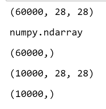
For example, if we feed an image which is 28 by 28 square in pixels and on the grey scale. This image will be a matrix of numbers in the below fashion-
28*28*1. Each of the 784 pixels can any values between 0-255 depending on the intensity of grey-scale.
Now let’s talk about what happens in a convolution layer. The main objective of this layer is to derive features of an image by sliding smaller matrix called kernel or filter over the entire image through convolution.
What is convolution? Convolution is taking a dot product between the filter and the local regions
Kernels can be many types such as edge detection, blob of color, sharpening, blurring etc. You can find some main kernels over here. Please note that we can specify the number of filters during the network training process, however network will learn the filters on its own.
As a result of this convolution layers, the network creates numbers of features maps. The size of feature maps depends on the # of filters (kernels), size of filters, padding (zero padding to preserve size), and strides (steps by which a filter scans the original image). Please note that a non linear activation function such Relu or Tanh is applied at each convolution layer to generate modified feature maps.
Pooling Layer– The arrays generated from the convolution layers are generally very big and hence pooling layer is used predominantly to reduce the feature maps and retain the most important aspect. In other words this facilitate “Downsampling” using algorithms such as max pooling or average pooling etc. Moreover, as the numbers of parameters in the network are truncated, this layer also helps in avoiding over fitting. It is common to have pooling layers in between different convolution layers.
Fully Connected Layer– This enables every neuron in the layers to be interconnected to the neurons from the previous and next layer to take the matrix inputs from the previous layers and flatten it to pass on to the output layer. Which in turn will make prediction such as classification probability.
Here is an excellent write-up which provides further details on all of the above steps.
Since we know enough about how a CNN works, let’s code now-
In this example, we will be working with MNIST dataset and build a CNN to recognize handwritten digits from 0-9. We will be using classification accuracy as a metric to evaluate the model’s performance. Please see link for MNIST CNN working
Please note that CNN need very high amount of computational power and memory and hence it’s recommended that you run this in GPUs or Cloud. CPUs may not be able to fit the model. Furthermore, you may need to reduce batch size to a lower level to ensure algorithm runs successfully.
As you can see, the above model gives 99%+ accuracy in the classification.
Forecasting is a technique that is used for a variety of different purposes and situations such as sales forecasting, operational and budget planning etc. Similarly there are a variety of different techniques such as moving averages, smoothening, ARIMA etc to statistically make a forecast.
In this article we will talk about an open source package called “Prophet” from Facebook which takes away the complexity of other techniques without compromising on accuracy of the forecast. The guiding principle of this approach is General Additive Models (GAMs). More on which can be found over here.
Let’s look at an example of how to deploy Prophet in Python.
Jupyter Notebook can be started using many ways, most common ones are-
From the Windows or Mac search interface. Type “Jupyter Notebook” and it should show you to application to start
From Anaconda prompt by typing “jupyter notebook” at the anaconda prompt
For high graphics display such as with plotly package, you are advised to start the jupyter notebook using the following command- “jupyter notebook –NotebookApp.iopub_data_rate_limit=1e10”
Jupyter Notebook Start from Anaconda for High Resolution Graphics
otherwise you can get an error message similar to the one shown below-
Markov chains or Markov models are statistical sequential models leveraging probability concepts to predict outcome. This model is named after a Russian mathematician Andrey Markov. The main guiding principle for Markov chains is that the probability of certain events to happen in the future depend on past events. They can be broken down into different categories-
First order Markov model- probability of next event depends on the current event
Second order Markov model- probability of the next event depends on the current and the previous event
A Hidden Markov Model ( HMM) is where the previous states from which the current state is generated are hidden or unobserved or unknown.
and so on…
Markov models have been proven to be very effective in sequential modeling such as-
Speech recognition
Handwriting recognition
Stock market forecasting
Online sales attribution to channels
etc.
Here is a pictorial depiction of HMM-
This link has a very good visual explanation of the Markov Models and guiding principles.
R has an in built package called “ChannelAttribution” for solving online multi channel attribution. This package has also an excellent explanation of the Markov Model and working example.
Python also has a library to build Markov models in Python.
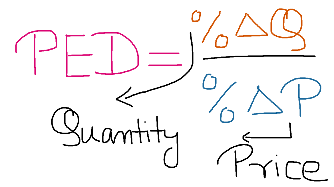
Price elasticity of demand (PED) is a measure that has been used in econometric to show how demand of a particular product changes when the price of the product is changed. More particularly, it measures the % change in demand of a product when the price changes by 1%.
It can be expressed as the following formula-
Let’s look at example- Let’s say that demand of a particular Bluetooth headset decreases by 2% when the price is increased by 1%. In this case the PED will be defined as = -2%/1% or -2.
Now, let’s talk about how we interpret PED-
PED of greater than 1 (absolute value) shows highly elastic product. In other words, the change in price will cause a more than proportionate change in demand. This is generally the case with non-essential or luxury products such as the example shown above. On the other hand, PED of less than 1 shows relatively inelastic products such as groceries and daily necessities. Furthermore, for most product PED will be negative, i.e. when the price is increased demand falls.
There are few other practical applications of PED that we should be aware of-
PED for a given product or product category can change over time and hence it’s imperative to measure PED over of time.
PED for a given product or product category can vary by customer segments. For example, low income customers may have higher PED for the same product
Pricing of a product should be optimized taking in account the PED. For example, if a product is showing lower price elasticity or inelasticity, pricing can be increased on the product to maximize revenue
Here is an article that gives some examples from the retail world.
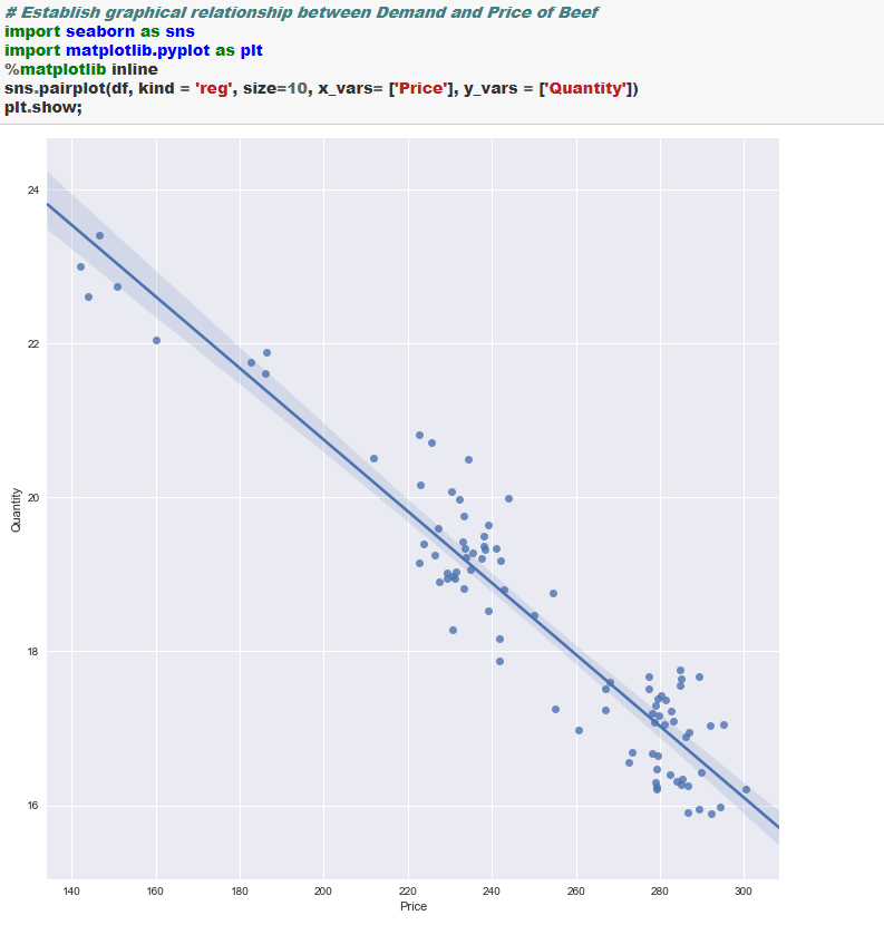
Let’s now step into how we can estimate PED in Python. For this, we will working with the beef price and demand data from USDA Red Meat Yearbook-
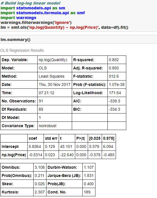
We will be building a log-log linear model to estimate PED. Please see here for the theoretical discussion on this topic. The coefficient from the log-log linear model shows the PED between two factors.
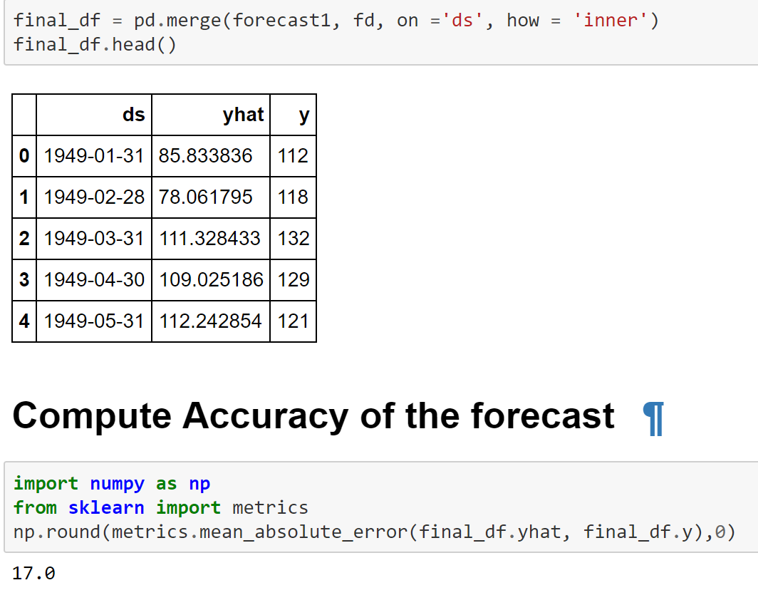
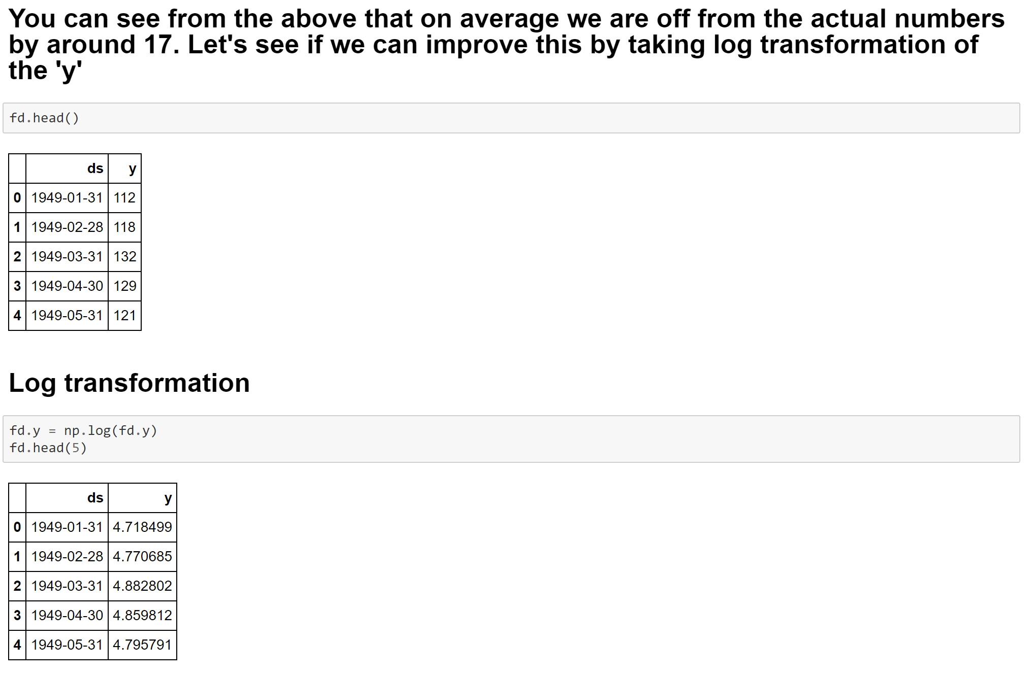
Let the Python show begin! In the below example PED comes out to be -0.53. It shows that when the price of beef is increased by 1% the demand for beef falls by 0.53%
The main objective of these recommendation systems is to do following-
Customization or personalizaiton
Cross sell
Up sell
Customer retention
Address the “Long Tail” phenomenon seen in Online stores vs Brick and Mortar stores
etc..
There are three main approaches for building any recommendation system-
Collaborative Filtering–
Users and items matrix is built. Normally this matrix is sparse, i.e. most of the cells will be empty. The goal of any recommendation system is to find similarities among the users and items and recommend items which have high probability of being liked by a user given the similarities between users and items.
Similarities between users and items can be assessed using several similarity measures such as Correlation, Cosine Similarities, Jaccard Index, Hamming Distance. The most commonly used similarity measures are Cosine Similarity and Jaccard Index in a recommendation engine
Content Based-
This type of recommendation engine focuses on finding the characteristics, attributes, tags or features of the items and recommend other items which have some of the same features. Such as recommend another action movie to a viewer who likes action movies.
Hybrid-
These recommendation systems combine both of the above approaches.
Build Recommendation System in Python using ” Scikit – Surprise”-
Now let’s switch gears and see how we can build recommendation engines in Python using a special Python library called Surprise.
This library offers all the necessary tools such as different algorithms (SVD, kNN, Matrix Factorization), in built datasets, similarity modules (Cosine, MSD, Pearson), sampling and models evaluations modules.
Here is how you can get started
Step 1- Switch to Python 2.7 Kernel, I couldn’t make it work in 3.6 and hence needed to install 2.7 as well in my Jupyter notebook environment
Step 2- Make sure you have Visual C++ compilers installed on your system as this package requires Cython Wheels. Here are couple of links to help you in this effort
Please note that if you don’t do the Step 2 correctly, you will get errors such as shown below – ” Failed building wheel for Scikit-surprise” or ” Microsoft Visual C++ 14 is required”
Step 3- Install Scikit- Surprise. Please make sure that you have Numpy installed before this
pip install numpy
pip install scikit-surprise
Step 4- Import scikit-surprise and make sure it’s correctly loaded


You must be logged in to post a comment.