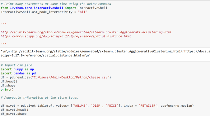
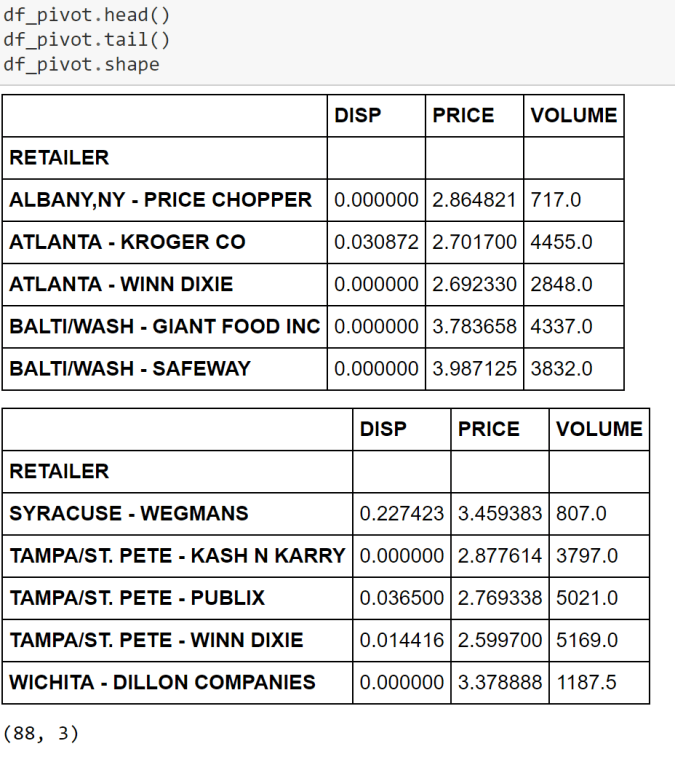
As highlighted in the article, clustering and segmentation play an instrumental role in Data Science. In this blog, we will show you how to build a Hierarchical Clustering with Python.
For this purpose, we will work with a R dataset called “Cheese”. Please install package called “Bayesm” in R and export this data set in csv format to be imported in Python. More on this dataset can be found here.
Overview: KMeans is an unsupervised machine learning algorithm used to partition data into a specified number of clusters (k). Each cluster is defined by its centroid, and the algorithm aims to minimize the distance between data points and their assigned cluster centroids.
Core Concepts:
Clusters and Centroids:
A cluster is a group of data points that are similar to each other.
The centroid is the mean position of all the points in a cluster.
Assignment and Update Steps:
Assignment: Each data point is assigned to the nearest centroid.
Update: The centroids are recalculated as the mean of all points assigned to each cluster.
Iterative Optimization:
The assignment and update steps are repeated until the centroids no longer change significantly or a maximum number of iterations is reached.
Assumptions:
The number of clusters (k) is known and fixed in advance.
Clusters are roughly spherical and equally sized.
Data points are closer to their own cluster centroid than to others.
The algorithm is sensitive to the initial placement of centroids.
Key Equations:
Distance Calculation:
The most common distance metric is Euclidean distance.
For a data point x and centroid c: Distance = sqrt( (x1 – c1)^2 + (x2 – c2)^2 + … + (xn – cn)^2 )
Centroid Update:
For each cluster, the new centroid is the mean of all points assigned to that cluster.
Centroid for cluster j: cj = (1 / Nj) * sum(xi) where Nj is the number of points in cluster j, and xi are the points in cluster j.
Objective Function (Inertia):
KMeans minimizes the sum of squared distances (inertia) between each point and its assigned centroid.
Inertia = sum over all clusters j [ sum over all points i in cluster j (distance(xi, cj))^2 ]
Algorithm Steps:
Choose k initial centroids (randomly or using a method like k-means++).
Assign each data point to the nearest centroid.
Recalculate centroids as the mean of assigned points.
Repeat steps 2 and 3 until centroids stabilize.
Limitations:
Sensitive to outliers and noise.
May converge to a local minimum (results can vary with different initializations).
Not suitable for clusters with non-spherical shapes or very different sizes.
Applications:
Market segmentation
Image compression
Document clustering
Anomaly detection
# Simple KMeans Clustering Example
import numpy as np
import matplotlib.pyplot as plt
from sklearn.datasets import make_blobs
from sklearn.cluster import KMeans
from sklearn.metrics import silhouette_score

# Generate synthetic data
X, y_true = make_blobs(n_samples=300, centers=4, cluster_std=0.60, random_state=42)

# Elbow method to find optimal k
inertia = []
k_range = range(1, 11)
for k in k_range:
    kmeans = KMeans(n_clusters=k, random_state=42)
    kmeans.fit(X)
    inertia.append(kmeans.inertia_)
plt.figure(figsize=(6,4))
plt.plot(k_range, inertia, 'bo-')
plt.axvline(x=4, color='red', linestyle='--', label='Optimal k=4')
plt.xlabel('Number of clusters (k)')
plt.ylabel('Inertia')
plt.title('Elbow Method for Optimal k')
plt.legend()
plt.grid(True)
plt.show()

# Fit KMeans with optimal k (choose visually, e.g., k=4)
k_opt = 4
kmeans = KMeans(n_clusters=k_opt, random_state=42)
labels = kmeans.fit_predict(X)

# Plot clusters
plt.figure(figsize=(7,5))
plt.scatter(X[:, 0], X[:, 1], c=labels, cmap='viridis', s=50)
plt.scatter(kmeans.cluster_centers_[:, 0], kmeans.cluster_centers_[:, 1], c='red', s=200, alpha=0.75, marker='X', label='Centers')
plt.title(f'KMeans Clustering (k={k_opt})')
plt.xlabel('Feature 1')
plt.ylabel('Feature 2')
plt.legend()
plt.show()

# Silhouette score
score = silhouette_score(X, labels)
print(f'Silhouette Score (k={k_opt}): {score:.3f}')
Silhouette Score (k=4): 0.876
# KMeans Clustering on Iris Dataset
import numpy as np
import matplotlib.pyplot as plt
from sklearn.datasets import load_iris
from sklearn.cluster import KMeans
from sklearn.metrics import silhouette_score
import pandas as pd
# Load Iris data
iris = load_iris()
X = iris.data
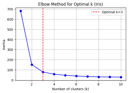
# Elbow method to find optimal k
inertia = []
k_range = range(1, 11)
for k in k_range:
kmeans = KMeans(n_clusters=k, random_state=42)
kmeans.fit(X)
inertia.append(kmeans.inertia_)
k_opt = 3 # Set optimal k explicitly for Iris data
plt.figure(figsize=(6,4))
plt.plot(k_range, inertia, 'bo-')
plt.axvline(x=k_opt, color='red', linestyle='--', label='Optimal k=3')
plt.xlabel('Number of clusters (k)')
plt.ylabel('Inertia')
plt.title('Elbow Method for Optimal k (Iris)')
plt.legend()
plt.grid(True)
plt.show()
# Fit KMeans with optimal k (choose visually, e.g., k=3)
kmeans = KMeans(n_clusters=k_opt, random_state=42)
labels = kmeans.fit_predict(X)
# Plot clusters (using first two features for visualization)
plt.figure(figsize=(7,5))
plt.scatter(X[:, 0], X[:, 1], c=labels, cmap='viridis', s=50)
plt.scatter(kmeans.cluster_centers_[:, 0], kmeans.cluster_centers_[:, 1], c='red', s=200, alpha=0.75, marker='X', label='Centers')
plt.title(f'Iris KMeans Clustering (k={k_opt})')
plt.xlabel(iris.feature_names[0])
plt.ylabel(iris.feature_names[1])
plt.legend()
plt.show()
# Plot clusters (using petal length and petal width for visualization)
plt.figure(figsize=(7,5))
plt.scatter(X[:, 2], X[:, 3], c=labels, cmap='viridis', s=50)
plt.scatter(kmeans.cluster_centers_[:, 2], kmeans.cluster_centers_[:, 3], c='red', s=200, alpha=0.75, marker='X', label='Centers')
plt.title(f'Iris KMeans Clustering (k={k_opt}) - Petal Length vs Petal Width')
plt.xlabel(iris.feature_names[2])
plt.ylabel(iris.feature_names[3])
plt.legend()
plt.show()
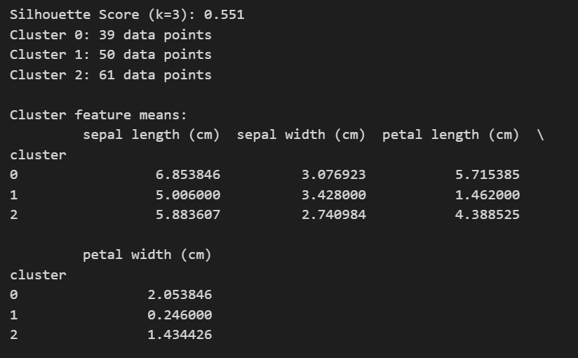
# Silhouette score
score = silhouette_score(X, labels)
print(f'Silhouette Score (k={k_opt}): {score:.3f}')
# Number of observations in each cluster
unique, counts = np.unique(labels, return_counts=True)
for i, count in zip(unique, counts):
print(f"Cluster {i}: {count} data points")
# Descriptive summary of each cluster (mean feature values)
df = pd.DataFrame(X, columns=iris.feature_names)
df['cluster'] = labels
print("\nCluster feature means:")
print(df.groupby('cluster').mean())


You must be logged in to post a comment.