Clean, text-free visual concept of Random Forest algorithm with multiple trees in an abstract style

Ensemble models are a great tool to fix the variance-bias trade-off which a typical machine learning model faces, i.e. when you try to lower bias, variance will go higher and vice-versa. This generally results in higher error rates.

Total Error in Model = Bias + Variance + Random Noise

Ensemble models typically combine several weak learners to build a stronger model, which will reduce variance and bias at the same time. Since ensemble models follow a community learning or divide and conquer approach, output from ensemble models will be wrong only when the majority of underlying learners are wrong.

One of the biggest flip side of ensemble models is that they may become “Black Box” and not very explainable as opposed a simple machine learning model. However, the gains in model performances generally outweigh any loss in transparency. That is the reason why you will see top performing models in many high ranking competitions will be generally an ensemble model.

Ensemble models can be broken down into the following three main categories-

Bagging
Boosting
Stacking

Let’s look at each one of them-

Bagging-

One good example of such model is Random Forest
These types of ensemble models work on reducing the variance by removing instability in the underlying complex models
Each learner is asked to do the classification or regression independently and in parallel and then either a voting or averaging of the output of all the learners is done to create the final output
Since these ensemble models are predominantly focuses on reducing the variance, the underlying models are fairly complex ( such as Decision Tree or Neural Network) to begin with low bias
An underlying decision tree will have higher depth and many branches. In other words, the tree will be deep and dense and with lower bias

Boosting-

Some good examples of these types of models are Gradient Boosting Tree, Adaboost, XGboost among others.
These ensemble models work with weak learners and try to improve the bias and variance simultaneously by working sequentially.
These are also called adaptive learners, as learning of one learner is dependent on how other learners are performing. For example, if a certain set of the data has higher mis-classification rate, this sample’s weight in the overall learning will be increased so that the other learners focus more on correctly classifying the tougher samples.
An underlying decision tree will be shallow and a weak learner with higher bias

There are various approaches for building a bagging model such as- pasting, bagging, random subspaces, random patches etc. You can find all details over here.

Stacking-

These meta learning models are what the name suggest. They are stacked models. Or in other words, a particular learner’s output will become an input to another model and so on.

How Ensembles Manage the Tradeoff

Ensemble	Examples	Fixes	Mechanism
Bagging	Random Forest	High variance	Many trees on bootstrap samples → average predictions
Boosting	XGBoost, Gradient Boosting	High bias	Weak learners trained sequentially on prior errors
Stacking	Meta-learner over base models	Both	Combines diverse models (e.g., logistic + tree + KNN)

Random Forest: Comprehensive Explanation

Core Concepts

Random Forest is an ensemble learning method that combines multiple decision trees to create a more robust and accurate predictive model. The algorithm works by building numerous decision trees and merging their predictions through voting (for classification) or averaging (for regression).

Key Principles

Bootstrap Aggregating (Bagging): Each tree in the forest is trained on a different bootstrap sample of the original dataset. This means each tree sees a slightly different version of the data, created by randomly sampling with replacement.

Feature Randomness: At each split in each tree, only a random subset of features is considered. This introduces additional randomness and helps prevent overfitting while reducing correlation between trees.

Ensemble Voting: For classification, each tree votes for a class, and the class with the most votes becomes the final prediction. For regression, predictions are averaged across all trees.

Core Assumptions

Independence of Errors: Individual trees should make different types of errors so that when combined, these errors cancel out
Feature Relevance: The dataset should contain features that are actually predictive of the target variable
Sufficient Data: There should be enough data to train multiple diverse trees effectively
Non-linear Relationships: Random forests can capture complex, non-linear relationships between features and targets

Key Equations and Formulas

Bootstrap Sample Size: Each bootstrap sample typically contains the same number of observations as the original dataset (n), created by sampling with replacement.

Number of Features at Each Split: For classification: sqrt(total_features), for regression: total_features/3

Final Prediction for Classification:
Prediction = mode(tree1_prediction, tree2_prediction, …, treeN_prediction)

Final Prediction for Regression:
Prediction = (tree1_prediction + tree2_prediction + … + treeN_prediction) / N

Out-of-Bag (OOB) Error: Each tree is tested on the ~37% of samples not included in its bootstrap sample, providing an unbiased estimate of model performance without needing a separate validation set.

Variable Importance: Calculated by measuring how much each feature decreases impurity when used for splits, averaged across all trees in the forest.

Advantages

Reduced Overfitting: Ensemble approach generalizes better than individual decision trees
Feature Importance: Provides natural feature importance scores
Handles Missing Values: Can maintain accuracy even with missing data
No Feature Scaling Required: Tree-based methods are not affected by feature scaling
Robust to Outliers: Tree splits are not heavily influenced by extreme values

End to End Python Execution-

			
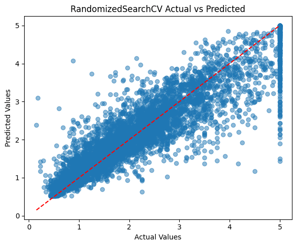
# - Random Forest Regression on California Housing Dataset
# - RandomizedSearchCV vs GridSearchCV:
# - GridSearchCV exhaustively tries every combination of hyperparameters in the provided grid.
# - RandomizedSearchCV samples a fixed number of random combinations from the grid, making it faster for large search spaces.
# - Both are used for hyperparameter optimization, but RandomizedSearchCV is more efficient when the grid is large or when you want a quick search.
import numpy as np  # For numerical operations
import pandas as pd  # For data manipulation
import matplotlib.pyplot as plt  # For plotting
import seaborn as sns  # For advanced visualizations
from sklearn.datasets import fetch_california_housing  # To load the dataset
from sklearn.model_selection import train_test_split, GridSearchCV, RandomizedSearchCV  # For splitting and hyperparameter search
from sklearn.ensemble import RandomForestRegressor  # Random Forest regression model
from sklearn.metrics import mean_squared_error, r2_score  # For regression metrics
import warnings  # To suppress warnings
warnings.filterwarnings('ignore')  # Ignore warnings for cleaner output
# Load California housing dataset
cal_data = fetch_california_housing()  # Fetch the dataset
X = pd.DataFrame(cal_data.data, columns=cal_data.feature_names)  # Features as DataFrame
y = cal_data.target  # Target variable (median house value)
# Train-test split
X_train, X_test, y_train, y_test = train_test_split(X, y, test_size=0.3, random_state=42)  # Split data into train and test sets
# Fixed lists for hyperparameters
param_list = {
    'n_estimators': [50, 100, 150, 200],  # Number of trees in the forest
    'max_depth': [5, 10, 15, None],  # Maximum depth of the tree
    'min_samples_split': [2, 4, 6, 8],  # Minimum samples required to split a node
    'min_samples_leaf': [1, 2, 3],  # Minimum samples required at a leaf node
    'max_features': ['sqrt', 'log2', None],  # Number of features to consider at each split
    'bootstrap': [True, False]  # Whether bootstrap samples are used
}
# RandomizedSearchCV for Random Forest Regressor
rf = RandomForestRegressor(random_state=42)  # Initialize Random Forest Regressor
random_search = RandomizedSearchCV(
    rf, param_distributions=param_list, n_iter=20, cv=3, scoring='neg_mean_squared_error', n_jobs=-1, random_state=42)  # Randomized hyperparameter search
random_search.fit(X_train, y_train)  # Fit model to training data
print('Best parameters (RandomizedSearchCV):', random_search.best_params_)  # Print best parameters
print('Best score (RandomizedSearchCV):', -random_search.best_score_)  # Print best score (MSE)
rf_random = random_search.best_estimator_  # Get best model
# GridSearchCV for Random Forest Regressor (commented out)
# grid_search = GridSearchCV(
#     rf, param_grid=param_list, cv=3, scoring='neg_mean_squared_error', n_jobs=-1)  # Grid hyperparameter search
# grid_search.fit(X_train, y_train)  # Fit model to training data
# print('Best parameters (GridSearchCV):', grid_search.best_params_)  # Print best parameters
# print('Best score (GridSearchCV):', -grid_search.best_score_)  # Print best score (MSE)
# rf_grid = grid_search.best_estimator_  # Get best model
# Evaluate RandomizedSearchCV model
y_pred = rf_random.predict(X_test)  # Predict on test set
mse = mean_squared_error(y_test, y_pred)  # Calculate mean squared error
r2 = r2_score(y_test, y_pred)  # Calculate R^2 score
print(f'\nRandomizedSearchCV Test MSE: {mse:.4f}')  # Print test MSE
print(f'RandomizedSearchCV Test R2: {r2:.4f}')  # Print test R^2
plt.figure(figsize=(6,5))  # Set figure size
plt.scatter(y_test, y_pred, alpha=0.5)  # Scatter plot of actual vs predicted
plt.plot([y_test.min(), y_test.max()], [y_test.min(), y_test.max()], 'r--')  # Diagonal reference line
plt.xlabel('Actual Values')  # X-axis label
plt.ylabel('Predicted Values')  # Y-axis label
plt.title('RandomizedSearchCV Actual vs Predicted')  # Plot title
plt.tight_layout()  # Adjust layout
plt.show()  # Show plot
# Feature importance visualization for best RandomizedSearchCV model
importances = rf_random.feature_importances_  # Get feature importances
indices = np.argsort(importances)[::-1]  # Sort features by importance
plt.figure(figsize=(8,5))  # Set figure size
plt.bar(range(X.shape[1]), importances[indices], align='center')  # Bar plot of importances
plt.xticks(range(X.shape[1]), [X.columns[i] for i in indices], rotation=45)  # Feature names as x-ticks
plt.title('Feature Importances (RandomizedSearchCV Best Model)')  # Plot title
plt.tight_layout()  # Adjust layout
plt.show()  # Show plot
# Visualize a single tree from the Random Forest
from sklearn.tree import plot_tree
plt.figure(figsize=(20,10))
plot_tree(rf_random.estimators_[0], feature_names=X.columns, filled=True, max_depth=2)
plt.title('Random Forest Regression: Example Tree (Depth=2)')
plt.show()

		

Best parameters (RandomizedSearchCV): {‘n_estimators’: 50, ‘min_samples_split’: 8, ‘min_samples_leaf’: 1, ‘max_features’: ‘log2’, ‘max_depth’: 15, ‘bootstrap’: False} Best score (RandomizedSearchCV): 0.26113711835896053 RandomizedSearchCV Test MSE: 0.2415 RandomizedSearchCV Test R2: 0.8160

			
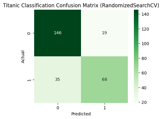
# Titanic Classification with Random Forest (Simplified)
import pandas as pd
import numpy as np
from sklearn.ensemble import RandomForestClassifier
from sklearn.model_selection import train_test_split, RandomizedSearchCV
from sklearn.metrics import accuracy_score, confusion_matrix, classification_report
from sklearn.preprocessing import LabelEncoder, StandardScaler
import seaborn as sns
import matplotlib.pyplot as plt
from sklearn.tree import plot_tree
# Load and preprocess Titanic dataset
X = sns.load_dataset('titanic').drop(['survived', 'deck', 'embark_town', 'alive', 'class', 'who'], axis=1)
X['age'] = X['age'].fillna(X['age'].median())
X['fare'] = X['fare'].fillna(X['fare'].median())
X['embarked'] = X['embarked'].fillna(X['embarked'].mode()[0])
X['alone'] = X['alone'].fillna(X['alone'].mode()[0])
for col in ['sex', 'embarked', 'alone']:
    X[col] = LabelEncoder().fit_transform(X[col])
X = X.drop(['adult_male'], axis=1)
scaler = StandardScaler()
X_scaled = scaler.fit_transform(X)
y = sns.load_dataset('titanic')['survived']
# Train-test split
X_train, X_test, y_train, y_test = train_test_split(X_scaled, y, test_size=0.3, random_state=42, stratify=y)
# Random Forest with RandomizedSearchCV
rf = RandomForestClassifier(random_state=42)
param_dist = {
    'n_estimators': [100, 200, 300],
    'max_depth': [5, 10, None],
    'min_samples_split': [2, 4, 6],
    'min_samples_leaf': [1, 2, 3],
    'max_features': ['sqrt', 'log2']
}
random_search = RandomizedSearchCV(rf, param_distributions=param_dist, n_iter=15, cv=3, scoring='accuracy', n_jobs=-1, random_state=42)
random_search.fit(X_train, y_train)
rf_best = random_search.best_estimator_
# Evaluation
y_pred = rf_best.predict(X_test)
print('Test Accuracy:', accuracy_score(y_test, y_pred))
print(classification_report(y_test, y_pred))
cm = confusion_matrix(y_test, y_pred)
plt.figure(figsize=(5,4))
sns.heatmap(cm, annot=True, fmt='d', cmap='Greens')
plt.title('Titanic Classification Confusion Matrix')
plt.xlabel('Predicted')
plt.ylabel('Actual')
plt.show()
# Feature importance
importances = rf_best.feature_importances_
indices = np.argsort(importances)[::-1]
plt.figure(figsize=(8,5))
plt.bar(range(X.shape[1]), importances[indices], align='center')
plt.xticks(range(X.shape[1]), [X.columns[i] for i in indices], rotation=45)
plt.title('Feature Importances (Titanic Random Forest)')
plt.tight_layout()
plt.show()
# Visualize tree with most important root split
root_feature = indices[0]
tree_idx = next((i for i, est in enumerate(rf_best.estimators_) if est.tree_.feature[0] == root_feature), 0)
plt.figure(figsize=(20,10))
plot_tree(rf_best.estimators_[tree_idx], feature_names=X.columns, filled=True, max_depth=2)
plt.title(f'Titanic Random Forest: Example Tree (Root={X.columns[root_feature]})')
plt.show()

		

Best parameters (RandomizedSearchCV): {‘n_estimators’: 200, ‘min_samples_split’: 2, ‘min_samples_leaf’: 1, ‘max_features’: ‘sqrt’, ‘max_depth’: 10} Best cross-validated accuracy (RandomizedSearchCV): 0.8378700606961477 Test Accuracy (RandomizedSearchCV): 0.7985074626865671

Cheers!

RP’s Blog on AI

Connect with RP- https://www.linkedin.com/in/ratnakarpandey/

Random Forest

Ensemble Modeling using Python

How Ensembles Manage the Tradeoff

Random Forest: Comprehensive Explanation

Core Concepts

Key Principles

Core Assumptions

Key Equations and Formulas

Advantages

How Ensembles Manage the Tradeoff

Random Forest: Comprehensive Explanation

Core Concepts

Key Principles

Core Assumptions

Key Equations and Formulas

Advantages

Share this: